Ingesting various events and documents into Elasticsearch is great for detailed analysis but when it comes to the common need to analyze data from a higher level, we need to aggregate the individual event data for more interesting insights. This is where Elasticsearch Data Frames come in.
Aggregation queries do a lot of this heavy lifting, but sometimes we need to prebake the aggregations for better performance and more options for analysis and machine learning.
In this lesson, we’ll explore how the Data Frames feature in Elasticsearch can help us create data aggregations for advanced analytics.
Elasticsearch Data Frame Transforms is an important feature in our toolbox that lets us define a mechanism to aggregate data by specific entities (like customer IDs, IP’s, etc) and create new summarized secondary indices.
Now, you may be asking yourself “with all the many aggregation queries already available to us, why would we want to create a new index with duplicated data?”
Why Elasticsearch Data Frames?
Transforms are definitely not here to replace aggregation queries, but rather to overcome the following limitations:
Performance: Complex dashboards may quickly run into performance issues as the aggregation queries get rerun every time, except if it’s cached. This can place excessive memory and compute demand on our cluster.
Result Limitations: As a result of performance issues, aggregations need to be bounded by various limits, but this can impact the search results to a point where we’re not finding what we want. For example, the maximum number of buckets returned, or the ordering and filtering limitations of aggregations.
Dimensionality of Data: For higher-level monitoring and insights, the raw data may not be very helpful. Having the data aggregated around a specific entity makes it easier to analyze and also enables us to apply machine learning to our data, like detecting outliers, for example.
How to Use Elasticsearch Data Frames
Let’s review how the Transform mechanism works.
Step 1: Define
To create a Transform you have two options either use Kibana or use the create transform API. We will later try both later, but we’ll dig deeper into the API.
There are four required parts of a Transform definition. You need to:
Provide an identifier (i.e. a name) which is a path parameter so it needs to comply with standard URL rules.
Specify the source index from which the “raw” data will be drawn
Define the actual transformation mechanism called a pivot which we will examine in a moment. If the term reminds you of a pivot table in Excel spreadsheets, that’s because it’s actually based on the same principle.
Specify the destination index to which the transformed data will be stored
Step 2: Run
Here, we have the option to run the transform one time with the Batchtransform, or we could run it on a scheduled basis using Continuous transform. We can easily preview our Transform before running it with the preview transform API.
If everything is ok, the Transform can be fired off with the start transform API, which will:
Create the destination index (if it doesn’t exist) and infer a target mapping
Perform assurance validations and run the transformation on the whole index or a subset of the data
This process ends up with the creation of what’s called a checkpoint, which marks what the Transform has processed. Continuous transforms, which run on a scheduled basis, create an incremental checkpoint each time the transform runs.
The Transformation Definition
The definition of the actual transformation has two key elements:
pivot.group_by is where you define one or more aggregations.
pivot.aggregations is where you define the actual aggregations you want to calculate in the buckets of data. For example, you can calculate the Average, Max, Min, Sum, Value count, custom Scripted metrics, and more.
Diving deeper into the pivot.group_by definition, we have a few ways we can choose to aggregate:
Terms: Aggregate data based on individual words that are found in your textual fields.
Histogram: Aggregate based on an interval of numeric values eg. 0-5, 5-10, etc.
Don’t worry if that doesn’t make full sense yet as now we’ll see how it works hands-on.
Hands-on Exercises
API
We will start with the API because generally, it’s more effective to understand the system and mechanics of the communication. From the data perspective, we’ll use an older dataset that was published by Elastic, the example NGINX web server logs.
The web server logs are extremely simple but are still close enough to real-world use cases.
Note: This dataset is very small and is just for our example, but the fundamentals remain valid when scaling up to actual deployments.
Let’s start by downloading the dataset to our local machine. The size is slightly over 11MB.
We will name our index for this data nginx and define its mapping. For the mapping we will map the time field as date (with custom format), remote_ip as ip, bytes as long and the rest as keywords.
Great! Now we need to index our data. To practice some valuable stuff, let’s use the bulk API and index all data with just one request. Although it requires some formal preprocessing, it’s the most efficient way to index data.
The preprocessing is simple as described by the bulk format. Before each document there needs to be an action defined (in our case just {“index”:{}}) and optionally some metadata.
This is basically a standard POST request to the _bulk endpoint. Also, notice the Content-Type header and the link to the file consisting of the processed data (prefixed with special sign @):
After few seconds, we have all our documents indexed and ready to play with:
vagrant@ubuntu-xenial:~/transforms$ curl localhost:9200/_cat/indices/nginx?v
health status index uuid                   pri rep docs.count docs.deleted store.size pri.store.size
green  open   nginx TNvzQrYSTQWe9f2CuYK1Qw   1   0      51462            0      3.1mb          3.1mb
Note: in relation to the data, as mentioned before, the dataset is of an older date so if you want to browse it in full be sure to set the dates in your queries or Kibana from between: ‘2015-05-16T00:00:00.000Z‘, to: ‘2015-06-04T23:30:00.000Z‘.
When the Transform is created, the transformation job is not started automatically, so to make it start we need to call the start Transform API like this:
vagrant@ubuntu-xenial:~/transforms$ curl --request POST 'http://localhost:9200/_transform/nginx_transform/_start'
>>>
{"acknowledged":true}
After a few moments, we should see the new index created filled with the aggregated data grouped by the remote_ip parameter.
Kibana
Via the Kibana interface, the Transform creation process is almost the same but maybe just more visually appealing so we won’t go into detail. But here are a few pointers to get you started.
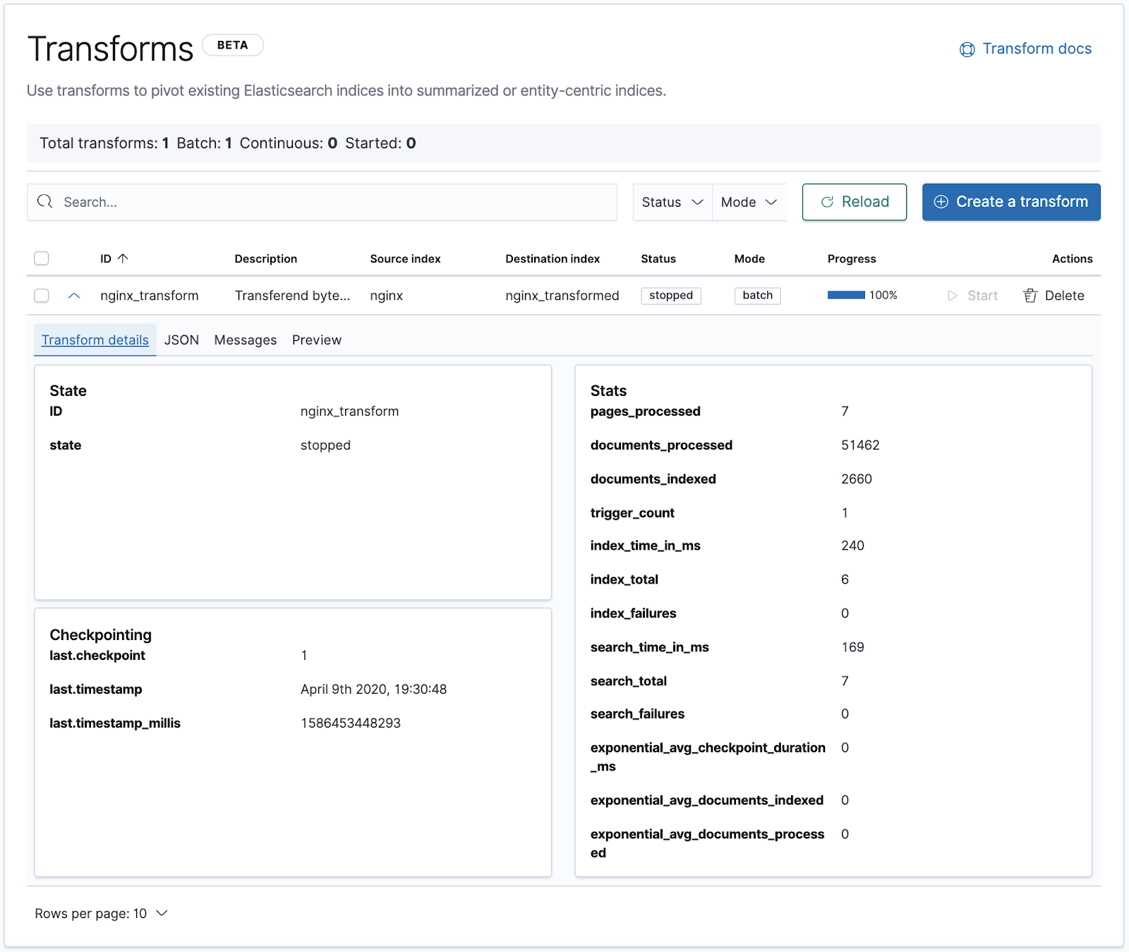
Start your journey in Management > Elasticsearch > Transforms section. By now, you should see our nginx_transform we created via the API and along with some detailed statistics on its execution.
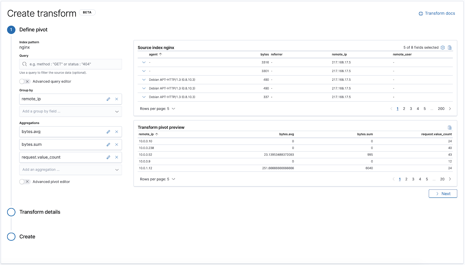
To create a new one, click the “Create a transform” button, pick a source index and start defining the Transform as we did with the API. Just be aware that the scripted aggregation would need to be defined in the Advanced pivot editor.
That’s it for Elasticsearch Data Frames! Now you can start running some truly insightful analysis.
In recent years, microservices have emerged as a popular architectural pattern. Although these self-contained services offer greater flexibility, scalability, and maintainability compared to monolithic applications, they…
Distributed microservices and cloud computing have been game changers for developers and enterprises. These services have helped enterprises develop complex systems easily and deploy apps faster….
Gaming apps are complex systems. They combine multi-function systems, like the game engine, to other resources such as server containers, proxies and CDNs in order to…
Where Modern Observability and Financial Savvy Meet.