PromQL Tutorial: 5 Tricks to Become a Prometheus God

For the seasoned user, PromQL confers the ability to analyze metrics and achieve high levels of observability. Unfortunately, PromQL has a reputation among novices for being a tough nut to crack.

Fear not! This PromQL tutorial will show you five paths to Prometheus godhood. Using these tricks will allow you to use Prometheus with the throttle wide open.

Aggregation

Aggregation is a great way to construct powerful PromQL queries. If you’re familiar with SQL, you’ll remember that GROUP BY allows you to group results by a field (e.g country or city) and apply an aggregate function, such as AVG() or COUNT(), to values of another field.

Aggregation in PromQL is a similar concept. Metric results are aggregated over a metric label and processed by an aggregation operator like sum().

Aggregation Operators

PromQL has twelve built in aggregation operators that allow you to perform statistics and data manipulation.

Group

What if you want to aggregate by a label just to get values for that label? Prometheus 2.0 introduced the group() operator for exactly this purpose. Using it makes queries easier to interpret and means you don’t need to use bodges.

Count those metrics

PromQL has two operators for counting up elements in a time series. Count() simply gives the total number of elements. Count_values() gives the number of elements within a time series that have a specified value. For example, we could count the number of binaries running each build version with the query: 

count_values("version", build_version)

Sum() does what it says. It takes the elements of a time series and simply adds them all together. For example if we wanted to know the total http requests across all our applications we can use:

sum(http_requests_total)

Stats

PromQL has 8 operators that pack a punch when it comes to stats. 

Avg() computes the arithmetic mean of values in a time series.

Min() and max() calculate the minimum and maximum values of a time series. If you want to know the k highest or lowest values of a time series, PromQL provides topk() and bottomk(). For example if we wanted the 5 largest HTTP requests counts across all instances we could write:

topk(5, http_requests_total)

Quantile() calculates an arbitrary upper or lower portion of a time series. It uses the idea that a dataset can be split into ‘quantiles’ such as quartiles or percentiles. For example, quantile(0.25, s) computes the upper quartile of the time series s.

Two powerful operators are stddev(), which computes the standard deviation of a time series and stdvar, which computes its variance.  These operators come in handy when you’ve got application metrics that fluctuate, such as traffic or disk usage.

By and Without

The by and without clauses enable you to choose which dimensions (metric labels) to aggregate along. by tells the query to include labels: the query sum by(instance) (node_filesystem_size_bytes) returns the total node_filesystem_size_bytes for each instance.

In contrast, without tells the query which labels not to include in the aggregation. The query sum without(job) (node_filesystem_size_bytes) returns the total node_filesystem_size_bytes for all labels except job.

Joining Metrics

SQL fans will be familiar with joining tables to increase the breadth and power of queries. Likewise, PromQL lets you join metrics. As a case in point, the multiplication operator can be applied element-wise to two instance vectors to produce a third vector.

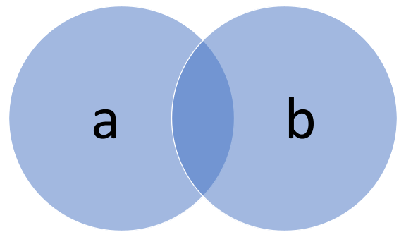
Let’s look at this query which joins instance vectors a and b.

a * b

This makes a resultant vector with elements a1b1, a2b2… anbn .  It’s important to realise that if a contains more elements than b or vice versa, the unmatched elements won’t be factored into the resultant vector.

This is similar to how an SQL inner join works; the resulting vector only contains values in both a and b.

Joining Metrics on Labels

We can change the way vectors a and b are matched using labels. For instance, the query a * on (foo, bar) group_left(baz) b matches vectors a and b on metric labels foo and bar. (group_left(baz) means the result contains baz, a label belonging to b.

Conversely you can use ignoring to specify which label you don’t want to join on. For example the query a * ignoring (baz) group_left(baz) b joins a and b on every label except  baz. Let’s assume a contains labels foo and bar and b contains foo, bar and baz. The query will join a to b on foo and bar and therefore be equivalent to the first query.

Later, we’ll see how joining can be used in Kubernetes.

Labels: Killing Two Birds with One Metric

Metric labels allow you to do more with less. They enable you to glean more system insights with fewer metrics.

Scenario: Using Metric Labels to Count Errors

Let’s say you want to track how many exceptions are thrown in your application. There’s a noob way to solve this and a Prometheus god way.

The Noob Solution

One solution is to create a counter metric for each given area of code. Each exception thrown would increment the metric by one.

This is all well and good, but how do we deal with one of our devs adding a new piece of code? In this solution we’d have to add a corresponding exception-tracking metric.  Imagine that barrel-loads of code monkeys keep adding code. And more code. And more code.

Our endpoint is going to pick up metric names like a ship picks up barnacles.  To retrieve the total exception count from this patchwork quilt of code areas, we’ll need to write complicated PromQL queries to stitch the metrics together.

The God Solution

There’s another way. Track the total exception count with a single application-wide metric and add metric labels to represent new areas of code. To illustrate, if the exception counter was called “application_error_count” and it covered code area “x”, we can tack on a corresponding metric label.

application_error_count{area="x"}

As you can see, the label is in braces.  If we wanted to extend application_error_count’s domain to code area “y”, we can use the following syntax.

application_error_count{area="x|y"}

This implementation allows us to bolt on as much code as we like without changing the PromQL query we use to get total exception count. All we need to do is add area labels.

If we do want the exception count for individual code areas, we can always slice application_error_count with an aggregate query such as:

count by(application_error_count)(area)

Using metric labels allows us to write flexible and scalable PromQL queries with a manageable number of metrics.

Manipulating Labels

PromQL’s two label manipulation commands are label_join and label_replace.  label_join allows you to take values from separate labels and group them into one new label. The best way to understand this concept is with an example.

label_join(up{job="api-server",src1="a",src2="b",src3="c"}, "foo", ",", "src1", "src2", "src3")

In this query, the values of three labels, src1, src2 and src3 are grouped into label foo. Foo now contains the respective values of src1, src2 and src3 which are a, b, and c.

label_replace renames a given label. Let’s examine the query

label_replace(up{job="api-server",service="a:c"}, "foo", "$1", "service", "(.*):.*")

This query replaces the label “service” with the label “foo”. Now foo adopts service’s value and becomes a stand in for it.  One use of label_replace is writing cool queries for Kubernetes.

Creating Alerts with predict_linear

Introduced in 2015, predict_linear is PromQL’s metric forecasting tool.  This function takes two arguments. The first is a gauge metric you want to predict. You need to provide this as a range vector. The second is the length of time you want to look ahead in seconds.

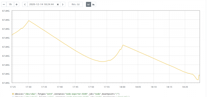
predict_linear takes the metric at hand and uses linear regression to extrapolate forward to its likely value in the future. As an example, let’s use PromLens to run the query: 

predict_linear(node_filesystem_avail_bytes{job="node"}[1h], 3600).

It shows a graph which shows the predicted value an hour from the current time.

Alerts and predict_linear

The main use of predict_linear is in creating alerts. Let’s imagine you want to know when you run out of disk space.  One way to do this would be an alert which fires as soon as a given disk usage threshold is crossed. For example, you might get alerted as soon as the disk is 80% full. 

Unfortunately, threshold alerts can’t cope with extremes of memory usage growth. If disk usage grows slowly, it makes for noisy alerts. An alert telling you to urgently act on a disk that’s 80% full is a nuisance if disk space will only run out in a month’s time.

If, on the other hand, disk usage fluctuates rapidly, the same alert might be a woefully inadequate warning. The fundamental problem is that threshold-based alerting knows only the system’s history, not its future.

In contrast, an alert based on predict_linear can tell you exactly how long you’ve got before disk space runs out. Plus, it’ll even handle left curves such as sharp spikes in disk usage.

Scenario: predict_linear in action

This wouldn’t be a good PromQL tutorial without a working example, so let’s see how to implement an alert which gives you 4 hours notice when your disk is about to fill up. You can begin creating the alert using the following code in a file “node.rules”.

- name: node.rules

  rules:

  - alert: DiskWillFillIn4Hours

    expr: predict_linear(node_filesystem_free{job="node"}[1h], 4*3600) < 0

    for: 5m

    labels:

      severity: page

The key to this is the fourth line.

expr: predict_linear(node_filesystem_free{job="node"}[1h], 4*3600) < 0

This is a PromQL expression using predict_linear. node_filesystem_free is a gauge metric measuring the amount of memory unused by your application. The expression is performing linear regression over the last hour of filesystem history and predicting the probable free space.  If this is less than zero the alert is triggered.

The line after this is a failsafe, telling the system to test predict_linear twice over a 5 minute interval in case a spike or race condition gives a false positive.

Using PromQL’s predict_linear function leads to smarter, less noisy alerts that don’t give false alarms and do give you plenty of time to act.

Putting it All Together: Monitoring CPU Usage in Kubernetes

To finish off this PromQL tutorial, let’s see how PromQL can be used to create graphs of CPU-utilisation in a Kubernetes application.

In Kubernetes, applications are packaged into containers and containers live on pods. Pods specify how many resources a container can use. If a container uses more resources than its pod has, it ‘spills over’ into a second pod.

This means that a candidate PromQL query needs the ability to sum over multiple pods to get the total resources for a given container. Our query should come out with something like the following.

Container	CPU utilisation per second
redash-redis	0.5
redash-server-gunicorn	0.1

Aggregating by Pod Name

We can start by creating a metric of CPU usage for the whole system, called container_cpu_usage_seconds_total.  To get the CPU utilisation per second for a specific namespace within the system we use the following query which uses PromQL’s rate function:

rate(container_cpu_usage_seconds_total{namespace= “redash”[5m])

This is where aggregation comes in. We can wrap the above query in a sum query that aggregates over the pod name.

sum by(pod_name)(

 rate(container_cpu_usage_seconds_total{namespace= “redash”[5m])

)

So far, our query is summing the CPU usage rate for each pod by name.

Retrieving Pod Labels

For the next step, we need to get the pod labels, “pod” and “label_app”. We can do this with the query:

group(kube_pod_labels{label_app=~”redash-*”}) by (label_app, pod)

By itself, kube_pod_labels returns all existing labels. The code between the braces is a filter acting on label_app for values beginning with “redash-”.

We don’t, however, want all the labels, just label_app and pod. Luckily, we can exploit the fact that pod labels have a value of 1. This allows us to use group() to aggregate along the two pod labels that we want. All the others are dropped from the results.

Joining Things Up

So far, we’ve got two aggregation queries. Query 1 uses sum() to get CPU usage for each pod.  Query 2 filters for the label names label_app and pod.  In order to get our final graph, we have to join them up. To do that we’re going to use two tricks, label_replace() and metric joining.

The reason we need label replace is that at the moment query 1 and query 2 don’t have any labels in common.  We’ll rectify this by replacing pod_name with pod in query 1. This will allow us to join both queries on the label “pod”. We’ll then use the multiplication operator to join the two queries into a single vector.

We’ll pass this vector into sum() aggregating along label app. Here’s the final query:

sum(

group(kube_pod_labels{label_app=~”redash-*”}) by (label_app, pod)

*

on (pod)

group_right(label_app)

label_replace

sum by(pod_name)(

 rate(container_cpu_usage_seconds_total{namespace= “redash”[5m])

), “pod”, “$1”, “pod_name”, “(.+)”

)by label_app

Hopefully this PromQL tutorial has given you a sense for what the language can do.  Prometheus takes its name from a Titan in Greek mythology, who stole fire from the gods and gave it to mortal man.  In the same spirit, I’ve written this tutorial to put some of the power of Prometheus in your hands.

You can put the ideas you’ve just read about into practice using the resources below, which include online code editors to play with the fire of PromQL at your own pace.

PromQL Tutorial Resources

PromLens

This online editor allows you to get started with PromQL without downloading Prometheus. As well as tabular and graph views, there is also an “explain” view. This gives the straight dope on what each function in your query is doing, helping you understand the language in the process.

Grafana Fundamentals

This tutorial by Coralogix explains how to integrate your Grafana instance with Coralogix, or you can use our hosted Grafana instance that comes automatically connected to your Coralogix data.

Prometheus on Coralogix

This tutorial will demonstrate how to integrate your Prometheus instance with Coralogix, to take full advantage of both a powerful open source solution and one of the most cutting edge SaaS products on the market.