SHAP: Are Global Explanations Sufficient in Understanding Machine Learning Predictions?

After training a machine learning (ML) model, data scientists are usually interested in the global explanations of model predictions i.e., explaining how each feature contributes to the model’s predictions over the entire training data. This is most important during the training and development stage of the MLOps lifecycle – for data scientists to understand their models, filter out unimportant features, obtain insights for feature engineering to improve model performance, and provide insights to stakeholders outside the data science team.

In light of all the aforementioned opportunities for global explainability, global explanations are limited in understanding the contribution of features to individual predictions.

For example, assume the following scenario:

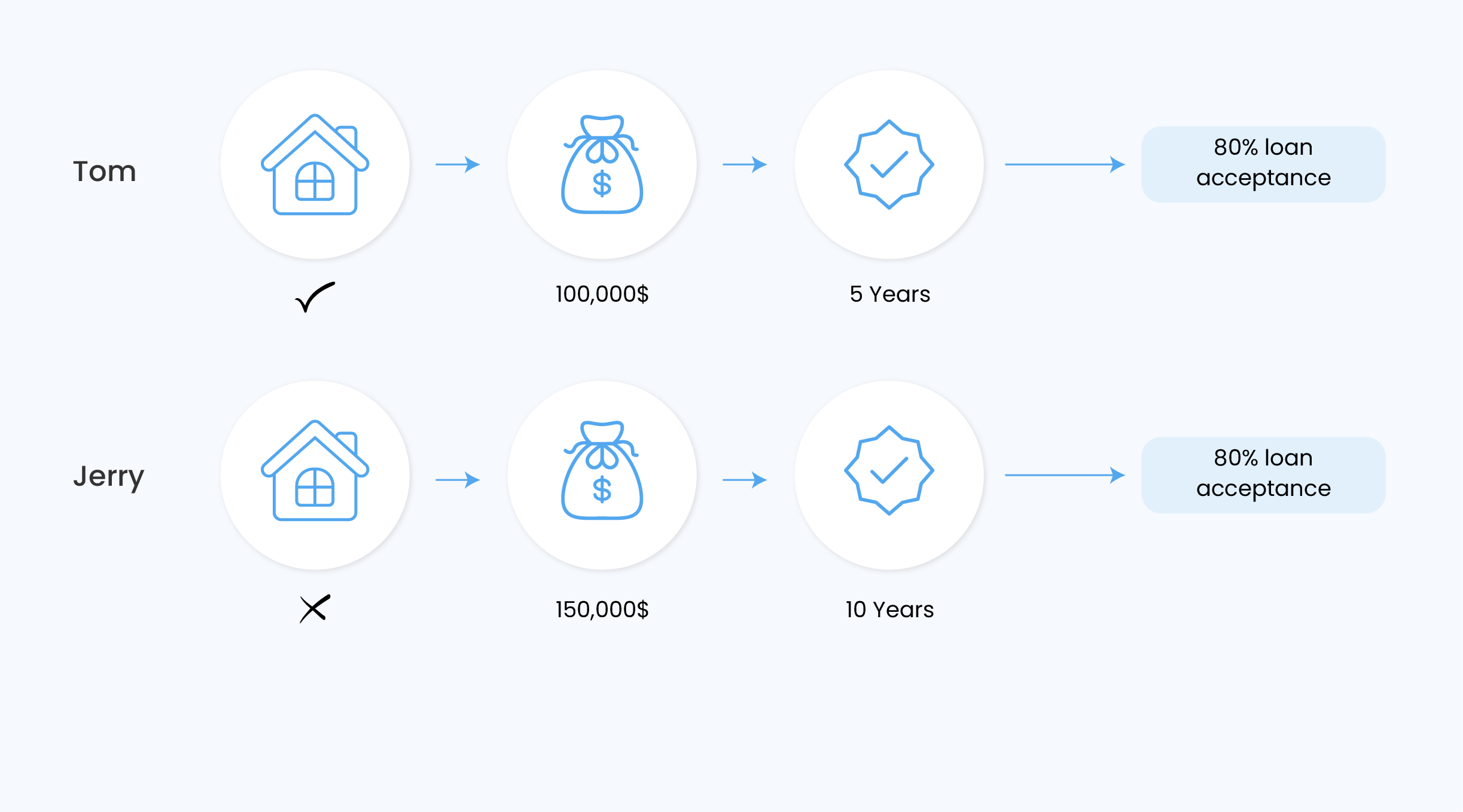
You train a machine learning model to predict the probability of a person getting a loan using the historical data of people who were accepted/rejected for loans. The data contains three features: house owner (Yes/No), income, and working experience. A global explainability technique, such as permutation importance is applied to understand the contribution of the features to the model’s predictions. The technique identifies income as the most important feature for accepting loans, however, two customers (Tom and Jerry) have similar probabilities of getting a loan with different incomes, working experience, and house ownership values. At this point, we need a local explainability technique to understand individual scenarios.

This article presents a state-of-the-art technique for local and instance-based machine learning explainability called SHAP (SHapley Additive exPlanations). The article targets senior data scientists and machine learning engineers who use SHAP but do not quite understand how the SHAP values are calculated. The remainder of the article is structured as followed:

1. Define SHAP and where it can be used within the MLOps lifecycle.
2. Describe how SHAP values are computed using our loan acceptance prediction problem.
3. Provide advantages and disadvantages of SHAP.

What is SHAP and When Can it Be Used?

SHAP is a machine learning explainability approach for understanding the importance of features in individual instances i.e., local explanations. SHAP comes in handy during the production and monitoring stage of the MLOps lifecycle, where the data scientists wish to monitor and explain individual predictions.

How are SHAP Values Calculated?

The SHAP value of a feature in a prediction (also known as Shapley value) represents the average marginal contribution of adding the feature to coalitions without the feature. For example, if we consider the following feature coalitions obtained from the loan acceptance problem.

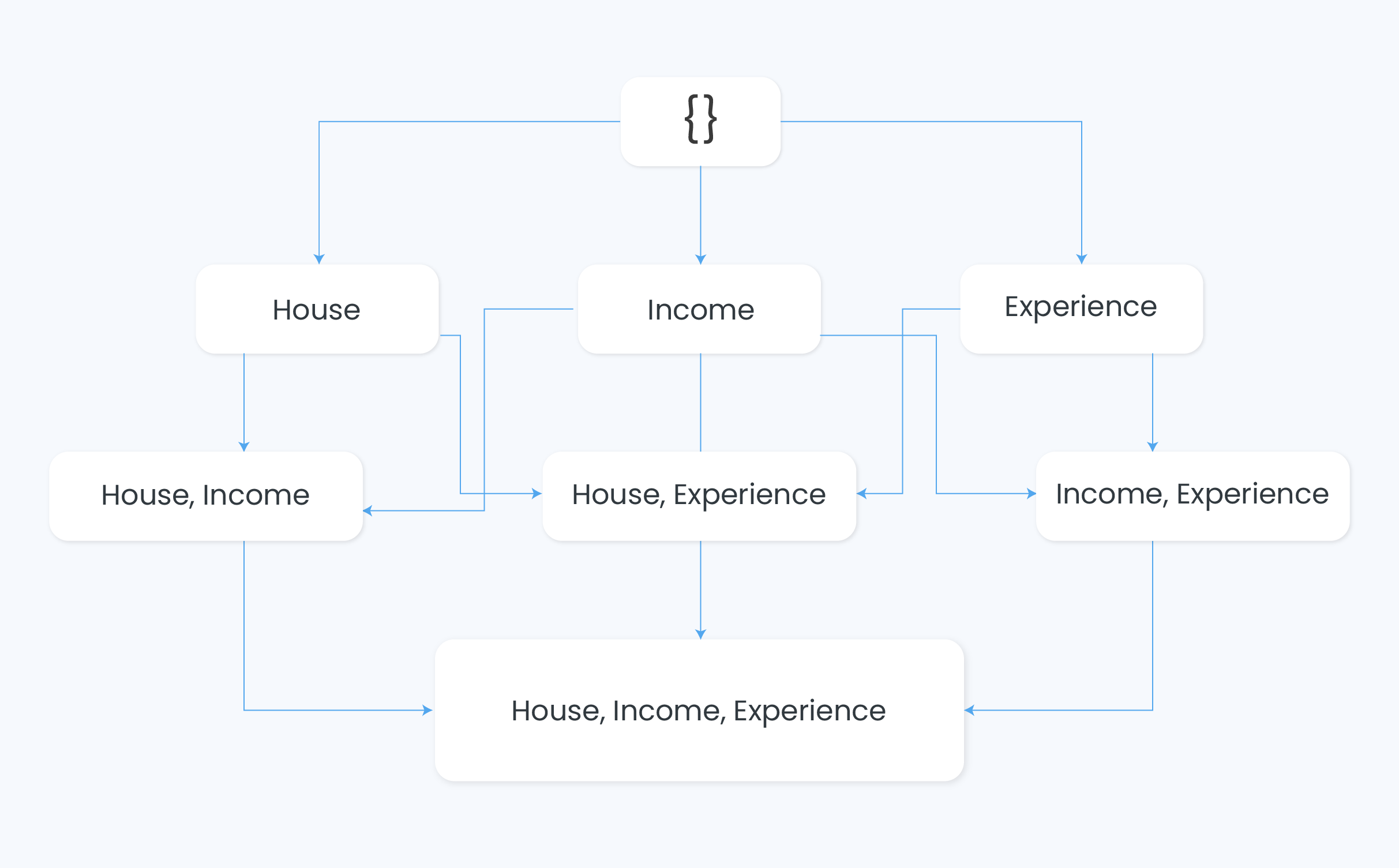
The contribution of owning a house in Tom’s 80% loan acceptance prediction will be the average marginal contribution when we add the feature to coalitions without a house indicated by the red edges in the coalition graph:

Therefore, the contribution of owning a house in Tom’s prediction can be computing using the following SHAP equation: 

[katex]SHAP(house) =[/katex]

[katex]w1 * frac{1}{n }sum_{i=1}^{n}Predict(house) – Predict({left { right }}) + [/katex]

[katex] w2* frac{1}{n }sum_{i=1}^{n}Predict(house,income) – Predict({income}) + [/katex]

[katex]w3* frac{1}{n }sum_{i=1}^{n}Predict(house,experience) – Predict({experience}) + [/katex]

[katex]w4* frac{1}{n }sum_{i=1}^{n}Predict(house,income,experience) – Predict({income, experience}) [/katex]

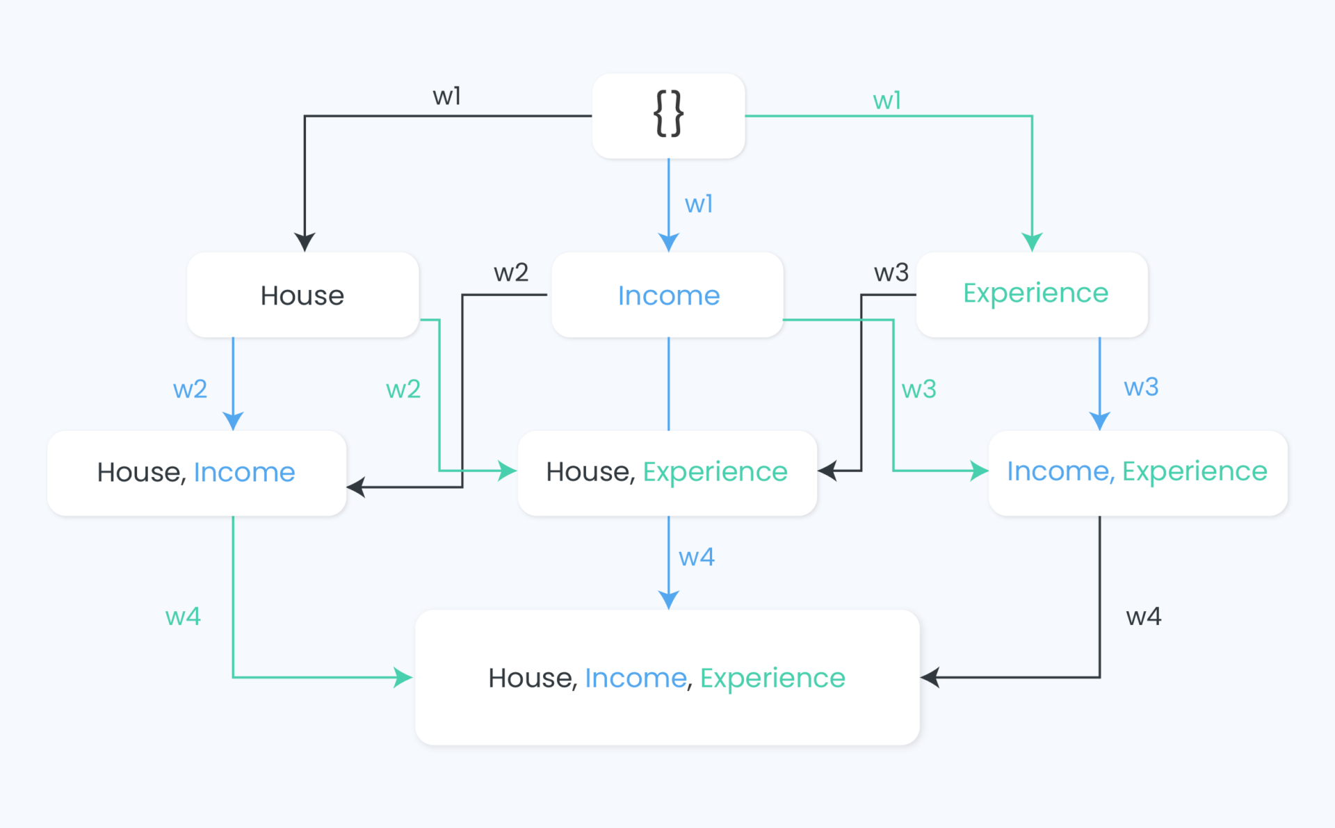
Where w is the weight for each marginal coalition determined by the number of edges in their level on the graph e.g., w1 = ⅓  and w3 = ⅙ ; and n is the number of randomly selected instances in the dataset to replace feature values in the coalition. 

Features present in a coalition use the feature values of the instance of interest, while the features absent in the coalition are replaced with feature values from random instances to calculate the predictions e.g., for  Predict(income, experience), only house value will be replaced by a value obtained from a random instance, and for Predict(experience), income and house values will be replaced. Therefore, to obtain the Shapley values for Income and Experience, we repeat the process of traversing the coalition graph from coalitions without the features to coalitions where the features are present and using the Shapley equation above. The blue path in our coalition graph represents the pathway for Income and the green for Experience.

Advantages of SHAP

• SHAP can be used for both local and global explanations. For global explanations, the absolute Shapley values of all instances in the data are averaged.
• SHAP shows the direction of impact of features on predictions i.e., negative and positive contributions.

Limitations of SHAP

• SHAP requires access to data as it randomly samples instances in the dataset to calculate the Shapley values.
• It can be very expensive in terms of computation time for datasets with many features as it requires all possible feature coalitions for its computation

Conclusion

This article provided detailed and mathematical illustrations of computing local explanations using SHAP. To summarize, SHAP sums up the marginal contribution of a feature by traversing the coalition graph from coalitions without the feature to coalitions where the feature is present. The marginal contributions are computed using random instances in the data. The key take-home message is that global explanations are important during model training and evaluation, while local explanations are important during model production and monitoring to understand individual predictions.

Alon Gubkin

Alon is the Chief Technology Officer and Co-Founder of Coralogix. Since building his first neuroevolution-based Super Mario bot in 2012 (which barely scratched the first level—too many 'hallucinations'...), he’s been fascinated by AI agents.