Kafka Streams Window By & RocksDB Tuning


Kafka Streams offers a feature called a window. In this post, I will explain how to implement tumbling time windows in Scala, and how to tune RocksDB accordingly.
Kafka Streams Terminology
- Clock Time: The operating system time of the consumer application.
- Record Timestamp: Each record in Kafka has a timestamp. If a timestamp was not defined when the record was produced into the topic, then the timestamp will be set to the clock time of the Kafka broker which initially received it.
- Stream Time: A separate Kafka Streams timestamp, which indicates the
latest Record Timestamp that Kafka Streams has encountered so far. - Event Time: A timestamp that exists inside the record’s Key or Value
- State Store: Like any Kafka Streams functionality, the accumulation is kept track of in a local database called a state store. (In our example we will use the reduce function and the ByteArrayWindowStore state store)
################## A note about record timestamps ##################
Kafka Streams retains the record timestamp of the record that was originally consumed, so that when topics like discussed windowed topic are produced, the record in the windowed topic will have the same record timestamp as the record in the original topic.
If you wouldn't find the original Record Timestamp to be valuable for your use-case, you can easily use the
Event Time
using a
TimestampExtractor
.
Data structure
In Kafka, each record has a key and a timestamp of when it was created. While Kafka can guarantee that all records will be delivered to topic consumers, Kafka can’t guarantee that all of the records will arrive in the chronological order of their timestamps. Thus, the Kafka topic consists of records that are chronologically unordered.
Let’s consider a stream of data records that are produced to a Kafka topic, in the order in which they will be consumed:
┌──────────┬────────────────────┐
│Record Key│  Record Timestamp  │
├──────────┼────────────────────┤
│    A     │         1          │
│          │                    │
│    B     │         2          │
│          │                    │
│    A     │         1          │
│          │                    │
│    B     │         1          │
│          │                    │
│    A     │         1          │
│          │                    │
│    .     │         .          │
│    .     │         .          │
│    .     │         .          │
│          │                    │
└──────────┴────────────────────┘
In this stream, first a record with key A is consumed with a timestamp of 1, then a record with key B is consumed with a timestamp of 2, and so on.
Kafka Streams allows us, through the windowing function, to construct a new topic which describes how frequently (count) each record (per Key) appears in the original topic.
How does this work? Let’s step through, record by record. After the first record (Key A with timestamp 1) is consumed, the new topic appears like this:
┌─────────┬────────────────────┬────────────────────┐
│Record ID│  Record Timestamp  │      Frequency     │
├─────────┼────────────────────┼────────────────────┤
│    A    │         1          │         1          │
└─────────┴────────────────────┴────────────────────┘
This is the first time that a record with Key A was encountered, so the new topic presents the record, its timestamp, and its frequency (1) accordingly.
Now let’s consume the next record (Key B with timestamp 2):
┌──────────┬────────────────────┬────────────────────┐
│Record Key│  Record Timestamp  │      Frequency     │
├──────────┼────────────────────┼────────────────────┤
│    A     │         1          │         1          │
│          │                    │                    │
│    B     │         2          │         1          │
└──────────┴────────────────────┴────────────────────┘
As this is the first time that we’ve consumed a record with Key B at all, it also shows up with a frequency of 1.
Now let’s consume the next record (Key A with timestamp 1):
┌──────────┬────────────────────┬────────────────────┐
│Record Key│  Record Timestamp  │      Frequency     │
├──────────┼────────────────────┼────────────────────┤
│    A     │         1          │         1          │
│          │                    │                    │
│    B     │         2          │         1          │
│          │                    │                    │
│    A     │         1          │         2          │
└──────────┴────────────────────┴────────────────────┘
This is the second time that our consumer has encountered a record with both a Key of A and a timestamp of 1, so this time, the resulting topic gives us an update — it tells us that a record with Key A and timestamp 1 has
appeared twice, hence the frequency value of 2.
Now let’s consume the next record (Key B with timestamp 1):
┌──────────┬────────────────────┬────────────────────┐
│Record Key│  Record Timestamp  │      Frequency     │
├──────────┼────────────────────┼────────────────────┤
│    A     │         1          │         1          │
│          │                    │                    │
│    B     │         2          │         1          │
│          │                    │                    │
│    A     │         1          │         2          │
│          │                    │                    │
│    B     │         1          │         1          │
└──────────┴────────────────────┴────────────────────┘
Although this is the second time which our consumer has encountered a record with a Key of B, it is still the first time which our consumer has encountered a record with the combination of a Key of B and a timestamp
of 1 (remember, the previous record with Key of B had a timestamp of 2).
Thus, the newest record in the resulting topic holds a Key of B, a timestamp of 1, and a frequency of 1.
Now let’s consume the next record (Key A with timestamp 1):
┌──────────┬────────────────────┬────────────────────┐
│Record Key│  Record Timestamp  │      Frequency     │
├──────────┼────────────────────┼────────────────────┤
│    A     │         1          │         1          │
│          │                    │                    │
│    B     │         2          │         1          │
│          │                    │                    │
│    A     │         1          │         2          │
│          │                    │                    │
│    B     │         1          │         1          │
│          │                    │                    │
│    A     │         1          │         3          │
└──────────┴────────────────────┴────────────────────┘
As we have now consumed 3 records with the combination of Key A and timestamp 1, the resulting topic now has a record that “updates” its consumers that the record with Key A, and timestamp 1, has appeared three times.
This “windowed topic” can thus give us statistical insights into our data, over a given window of time.
Windowing Terminology
- Window: the timeframe size Kafka Streams should accumulate statistics over
- Grace Period: how long Kafka Streams should consider a record to still be statistically valuable, after which the window will be “closed” and the record will be discarded.
- Discarded Records: once the window is closed (i.e. the Window and Grace Period has passed) every record that matches a “closed” window is silently dropped and ignored.
Example
Consider the following topic:
┌──────────┬────────────────────┐
│Record Key│  Record Timestamp  │
├──────────┼────────────────────┤
│    A     │         1          │
│          │                    │
│    A     │         1          │
│          │                    │
│    A     │         1          │
│          │                    │
│    A     │         7          │
│          │                    │
│    A     │         9          │
│          │                    │
│    A     │         1          │
│          │                    │
│    .     │         .          │
│    .     │         .          │
│    .     │         .          │
│          │                    │
└──────────┴────────────────────┘
If we use the same accumulation function as before, a window of 5, and an infinite grace period, then Kafka Streams will produce the following windowed topic:
┌──────────┬────────────────────┬────────────────────┬────────────────────┐
│Record Key│  Record Timestamp  │      Frequency     │    Window Frame    │
├──────────┼────────────────────┼────────────────────┼────────────────────┤
│    A     │         1          │         1          │      1 - 6         │
│          │                    │                    │                    │
│    A     │         1          │         2          │      1 - 6         │
│          │                    │                    │                    │
│    A     │         1          │         3          │      1 - 6         │
│          │                    │                    │                    │
│    A     │         7          │         1          │      7 - 12        │
│          │                    │                    │                    │
│    A     │         9          │         2          │      7 - 12        │
│          │                    │                    │                    │
│    A     │         1          │         4          │      1 - 6         │
│          │                    │                    │                    │
└──────────┴────────────────────┴────────────────────┴────────────────────┘
In this windowed topic, the first three records show an increasing frequency, as a record with Key A and timestamp 1 showed up four times. Then a record with a timestamp of 7 appeared, then a record with a timestamp of 9 appeared, but related to the same timeframe so their frequency is 2.
Now, let’s assume that instead of an infinite grace period, we define a grace period of 2. The resulting windowed topic will be:
┌──────────┬────────────────────┬────────────────────┐
│Record Key│  Record Timestamp  │      Frequency     │
├──────────┼────────────────────┼────────────────────┤
│    A     │         1          │         1          │
│          │                    │                    │
│    A     │         1          │         2          │
│          │                    │                    │
│    A     │         1          │         3          │
│          │                    │                    │
│    A     │         7          │         1          │
│          │                    │                    │
│    A     │         9          │         2          │
│          │                    │                    │
└──────────┴────────────────────┴────────────────────┘
Note that this is exactly the same topic, except that the final record, with Key A, timestamp 1, and frequency 4, no longer appears.
Because 6+2=8, a window with a timeframe of 1–6and grace time is 8 (earlier than 9) is considered to be so old as to be irrelevant, and it is no longer tracked in the windowed topic.
Coding (!)
Requirements:
Scala 2.13
Kafka Streams 2.5.0
Topology
Topology Constants
Constants
import org.apache.kafka.streams.scala.StreamsBuilder
val builder = new StreamsBuilder()
val storeName = "reducer-store-name"
val sourceTopic = "input-topic"
val sinkTopic = "output-topic"
val gracePeriod = 6.hours
val windowSize = 1.minute
Configure State Store
State Store
import org.apache.kafka.streams.scala.kstream.Materialized
import org.apache.kafka.streams.scala.ByteArrayWindowStore

val store = Materialized
  .as[Key, Long, ByteArrayWindowStore](storeName)
  .withRetention(gracePeriod.plus(windowSize))
- withRetention — sets the retention period for the state store. This is the minimum amount of time that Kafka Streams should hold onto records for, so it is set to window plus grace.
- storeName — is used by Kafka Streams to determine the filesystem path to which the store will be saved to, and let us configure RocksDB for this specific state store.
Create grouped by Key source
Source
val kGroupedStream = builder
  .stream[Key, Long](sourceTopic)
  .groupByKey
- stream: Create an input stream from the topic sourceTopic, using Key and Long Serdes.
- groupByKey: In order to create window operations on a stream of records with keys, it’s necessary to use a KGroupedStream, not a KStream. This is done by calling groupByKey on the KStream returned by stream.
Time Windowed KStream
Time Windowed
val timeWindowedKStream = kGroupedStream
  .windowedBy(
    TimeWindows
      .of(window)
      .grace(gracePeriod)
  )
- windowedBy: Create a new instance of TimeWindowedKStream that can be used to perform windowed aggregations.
- TimeWindows.of: Creates a window with the given window size
- grace: Returns a window with a grace by the given gracePeriod size
Accumulate windowed keys values
Accumulate
val windowedKTable = timeWindowedKStream
  .reduce(_ + _)(store)
- reduce: Each record with the same key and in each window will be reduced using the given function. In this example, the values of each record are added to each other.
- store: Store the reduced values in the preconfigured state store.
Produce Results
Produce
windowedKTable
  .toStream
  .to(sinkTopic)
- toStream: Creates a KStream from the KTable that was returned by the reduction.
- to: Produces the records to the topic sinkTopic (i.e. our windowed topic).
RocksDB Tuning
It’s important to remember that Kafka Streams uses RocksDB to power its local state stores.
Because RocksDB is not part of the JVM, the memory it’s using is not part of the JVM heap. If you’re not careful, you can very quickly run out of memory.
For our use-case at Coralogix, we need to use a combination of a fairly large grace period with a small window. In our experience, this caused RocksDB to use much more memory than we expected — upwards of 10 GB of RAM, even as CPU only increased marginally, by 6–7%. We wanted to find a way to decrease the amount of memory that RocksDB needed, but without causing a big increase in needed CPU as a result.
With some fine-tuning, I succeeded in lowering our memory usage to a maximum of 3 GB, while only increasing CPU to an average of 10%, and a maximum of 20%.
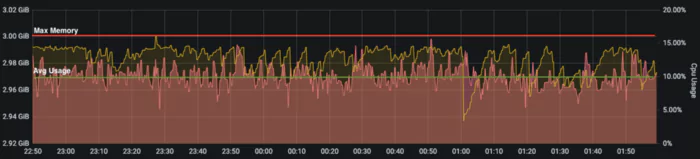
Memory and CPU usage
RocksDB Configurations
RocksDB Configuration
object BoundedMemoryRocksDBConfig {
  val storeName = ???
  val lruCacheBytes = 100L * 1024L * 1024L
  val maxBackgroundCompactions = 10
  val maxBackgroundFlushes = 10
  val maxBackgroundJobs = 20
  val memtableBytes = 1024 * 1024
  val nMemtables = 1
  val writeBufferManagerBytes = 95 * 1024 * 1024

  private val cache = new LRUCache(config.lruCacheBytes)
  private val writeBufferManager =
    new WriteBufferManager(writeBufferManagerBytes, cache)
}

class BoundedMemoryRocksDBConfig extends RocksDBConfigSetter {
  override def setConfig(
    storeName: String,
    options: Options,
    configs: util.Map[String, AnyRef]
  ): Unit =
    if (storeName.contains(BoundedMemoryRocksDBConfig.storeName)) {
      val tableConfig = options.tableFormatConfig.asInstanceOf[BlockBasedTableConfig]
      tableConfig.setBlockCache(BoundedMemoryRocksDBConfig.cache)
      tableConfig.setCacheIndexAndFilterBlocks(true)

      options
        .setWriteBufferManager(BoundedMemoryRocksDBConfig.writeBufferManager)
        .setMaxWriteBufferNumber(BoundedMemoryRocksDBConfig.nMemtables)
        .setWriteBufferSize(BoundedMemoryRocksDBConfig.memtableBytes)
        .setTableFormatConfig(tableConfig)
        .setMaxBackgroundCompactions(BoundedMemoryRocksDBConfig.maxBackgroundCompactions)
        .setMaxBackgroundFlushes(BoundedMemoryRocksDBConfig.maxBackgroundFlushes)
        .setMaxBackgroundJobs(BoundedMemoryRocksDBConfig.maxBackgroundJobs)
    }
  override def close(storeName: String, options: Options): Unit = {}
}
Additionally, we set up the JVM’s Xms and Xmx values to 1024m, and used the resource limits in Kubernetes to set a maximum limit of no more than 3 GB of memory.
Now, let’s dig a bit deeper into these configurations:
- lruCacheBytes: Used to create a Least Recently Used cache for reading and writing
- maxBackgroundCompactions: Increase the maximum concurrent background compactions
- maxBackgroundFlushes: Increase the maximum concurrent background flushes
- maxBackgroundJobs: Increase the maximum concurrent background jobs (both compactions and flushes)
- memtableBytes: The amount of data allowed to build up in memory before
writing to a sorted file on-disk - nMemtables: The maximum number of buffers that are built up in memory
- writeBufferManagerBytes: The maximum amount of memory to use across all buffers (write cache)
Therefore, the maximum memory calculation is as follows:
Maximum RAM = ((number of partitions) * lruCacheBytes) + (JVM -Xmx value)
So why did we change all of the other parameters?
We can affect the CPU usage by deciding to reduce (or increase) the number of writes to disk.
- A smaller writeBufferManagerBytes will cause the write buffer to fill up faster; when the write buffer is full, it will be flushed to disk.
- A smaller memtableBytes will also cause the write buffer to fill up faster and cause the write buffer to thus be flushed to disk more often.
If you encounter high CPU usage, you should increase the buffer sizes (up to lruCacheBytes), so that the disk will be flushed less frequently. However, remember that increasing lruCacheBytes (so that you can increase the buffer sizes further) will cause an increase in memory usage, which may eventually cause your application to reach OutOfMemory if you do not increase the memory limits accordingly.
You should also pay attention to how your data is sorted. In our case, we know to expect that records with the same ID and Record Timestamp should arrive at about the same time. This allows us to decrease the Read/Write cache ratio to only 5% for Reads and 95% for Writes, preserving availability for producers while spending the minimum amount of memory on aggregations (since it’s highly unlikely for records to arrive very late after their period of relevancy).
If you see high CPU usage, even when your windows and grace periods are smaller, you can change the ratio by setting writeBufferManagerBytes to a lower value, which will give more cache for reads.
It is an exciting time to join Coralogix’s engineering team. If this sounds interesting to you, please take a look at our job page — Work at Coralogix. If you’re particularly passionate about stream architecture, you may want to take a look at these two openings first: FullStack Engineer and Backend Engineer.
Further Reads
- Write Buffer Manager
- Memtable/Write Buffer
- RocksDB Memory usage
- RocksDB Options Class
- Block-Based Table Config
- Kafka Streams Tumbling time windows
- Kafka Streams Memory Management