Improve Elasticsearch Query Performance with Profiling and Slow Logs


If our end users end up too long for a query to return results due to Elasticsearch query performance issues, it can often lead to frustration. Slow queries can affect the search performance of an ecommerce site or a Business Intelligence dashboard – either way, this could lead to negative business consequences. So it’s important to know how to monitor the speed of search queries, diagnose and debug to improve search performance.
We have two main tools at our disposal to help us investigate and optimize the speed of Elasticsearch queries: Slow Log and Search Profiling.
Let’s review the features of these two instruments, examine a few use cases, and then test them out in our sandbox environment.
With sufficiently complex data it can be difficult to anticipate how end users will interact with your system. We may not have a clear idea of what they are searching for, and how they perform these searches. Because of this, we need to monitor searches for anomalies that may affect the speed of applications in a production environment. The Slow Log captures queries and their related metadata when a specified processing time exceeds a threshold for specific shards in a cluster.
Slow Log
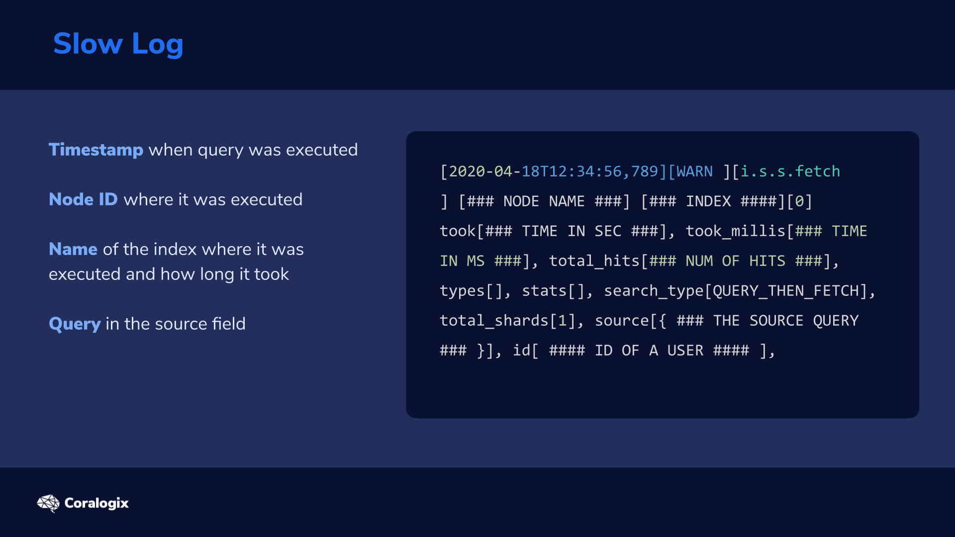
Here’s a sample slow log entry is as follows:
[2020-04-18T12:34:56,789][WARN ][i.s.s.fetch ] [### NODE NAME ###] [### INDEX ####][0] took[### TIME IN SEC ###], took_millis[### TIME IN MS ###], total_hits[### NUM OF HITS ###], types[], stats[], search_type[QUERY_THEN_FETCH], total_shards[1], source[{ ### THE SOURCE QUERY ### }], id[ #### ID OF A USER #### ],
Data in these logs consists of:
- Timestamp when the query was executed (for instance, for tracking the time of day of certain issues)
- Node ID
- Name of the index where it was executed and how long it took
- Query in the source field
The Slow Log also has a JSON version, making it possible to fetch these logs into Elasticsearch for analysis and displaying in a dashboard.
Search Profiling
When you discover Elasticsearch query performance issues in the Slow Log, you can analyze both the search queries and aggregations with the Profile API. The execution details are a fundamental aspect of Apache Lucene which lies under the hood of every shard, so let’s explore the key pieces and principles of the profiling output.
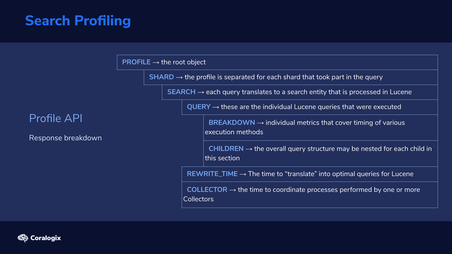
Let’s break down the response from the Profile API when it’s enabled on a search query:
| PROFILE → the root object consisting of the full profiling payload. | ||||
| array | SHARD → the profile is separated for each shard that took part in the query (we will be testing on a single-node single-shard config). | |||
| array | SEARCH → each query translates to a search entity that is processed in Lucene (Note: in most cases there will only be one). | |||
| array | QUERY → these are the individual Lucene queries that were executed. Important: these are usually not mapped 1:1 to the original Elasticsearch query, as the structure of Lucene queries is different. For example: a match query on two terms (e.g. “hello world”) will be translated to one boolean query with two term queries in Lucene. |
|||
| object | BREAKDOWN → individual metrics that cover timing of various execution methods in the Lucene index and the count of how many times they were executed. These can include scoring of a document, getting a next matching document etc. | |||
| array | CHILDREN → the overall query structure may be nested. You will find a breakdown for each child in this section. | |||
| value | REWRITE_TIME → as mentioned earlier, the Elasticsearch query undergoes a “translation” process into optimal queries for Lucene to execute. This process can have many iterations; the overall time is captured here. | |||
| array | COLLECTOR → the coordination process is performed by one or more Collectors. It provides a collection of matching documents, and performs additional aggregations, counting, sorting, or filtering on the result set. Here you find the time of execution for each process. | |||
| array | 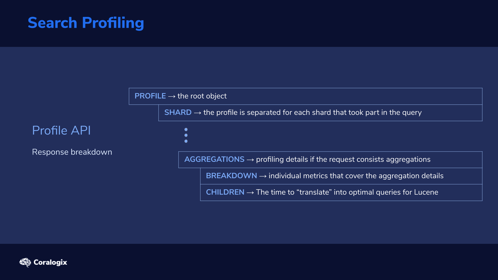
AGGREGATIONS → includes the profiling details if the request consists of one or more aggregations. |
|||
| object | BREAKDOWN → individual metrics that cover the aggregation details (such as initializing the aggregation, collecting the documents etc.). Note: the reduction phase is a summary of activity across shards. | |||
| array | CHILDREN → like queries, aggregations can be nested. | |||
There’s two important points to keep in mind with Search Profiling:
- These are not end-to-end measurements but only capture shard-level processing. The coordinating node work is not included, nor is any network latency, etc.
- Because profiling is a debugging tool it has a very large overhead so it’s typically enabled for a limited time to debug.
Search profiling can also be visualized in Kibana DevTools for easier analysis of the profiling responses. We’ll examine this later in the hands-on section.
Hands-on: Solving Elasticsearch Query Performance
First we need some data to play with. We’ll use a data set including the Wikipedia page data provided on the Coralogix github (more info on this dataset can be found in this article). While this is not a particularly small dataset (100 Mb), it still won’t reach the scale that you’re likely to find in many real-world applications which can consist of tens of GBs, or more.
To download the data and index them into our new wiki index, follow the commands below.
mkdir profiling && cd "$_"

for i in {1..10}
do
   wget "https://raw.githubusercontent.com/coralogix-resources/wikipedia_api_json_data/master/data/wiki_$i.bulk"
done

curl --request PUT 'https://localhost:9200/wiki'
--header 'Content-Type: application/json'
-d '{"settings": { "number_of_shards": 1, "number_of_replicas": 0 }}'

for bulk in *.bulk
do
   curl --silent --output /dev/null --request POST "https://localhost:9200/wiki/_doc/_bulk?refresh=true" --header 'Content-Type: application/x-ndjson' --data-binary "@$bulk"
   echo "Bulk item: $bulk INDEXED!"
done
As you can see we are not defining a specific mapping; we are using the defaults. We will then loop through the 10 bulk files downloaded from the repo and use the _bulk API to index them.
You can get a sense of what this dataset is about with the following query:
curl --location --request POST 'https://localhost:9200/wiki/_search?pretty' --header 'Content-Type: application/json' --data-raw '{
   "size": 1,
   "query": { "match": { "displaytitle": "cloud" } }
}'
Slow Log
For the slow log, we can customize a threshold that triggers a slow log to be stored with the following dynamic settings (dynamic means that you can effectively change them without restarting the index).
You can define standard log levels (warn/info/debug/trace) and also separate the query phase (documents matching and scoring) from the fetch phase (retrieval of the docs).
curl --request PUT 'https://localhost:9200/wiki/_settings'
--header 'Content-Type: application/json'
-d '{
   "index.search.slowlog.threshold.query.warn": "10ms",
   "index.search.slowlog.threshold.fetch.warn": "5ms",
   "index.search.slowlog.level": "info"
}'
Be aware that the query phase normally takes much longer to execute in a real-world production environment than what we see here.
If you use the default Elasticsearch installation you can find the Slow Log in the /var/log/elasticsearch directory:
sudo -su elasticsearch
ls /var/log/elasticsearch/ | grep search_slowlog
>>>
yourclustername_index_search_slowlog.json
yourclustername_index_search_slowlog.log
To reset the settings back to the default settings just pass in null instead of any value. The same is true for all other dynamic settings.
Profiling – API
Now let’s test the Profile API. We will store the results in a variable, so that we can play with them later.
Let’s compose a more complex query to see the resulting structure.
profile_result="$(curl --silent --location --request POST 'https://localhost:9200/wiki/_search?pretty' --header 'Content-Type: application/json' --data-raw '{
   "profile": true,
   "query": {
       "bool": {
           "should": {
               "multi_match": {
                   "fields": ["displaytitle", "description", "extract"],
                   "query": "database"
               }
           },
           "must": {
               "match_phrase": {
                   "extract": {
                       "query": "cloud service",
                       "slop": 2
                   }
               }
           },
           "filter" : {
               "range" : {
                   "timestamp" : { "gte" : "now-1y" }
               }
           }
       }
   }
}')"
Notice that the profile parameter is set to true. In this query, we’re searching for “cloud services.” We want to see them appear higher in the results than those that are related to “databases.” We also do not want results with a timestamp older than a year.
We can echo and grep the key profiling results:
echo "$profile_result" | jq '.profile.shards[].searches[].query[]' | grep 'type|description|time_in_nanos'
As you can see in the results, the original query was rewritten to a different structure but with the shared common boolean query.
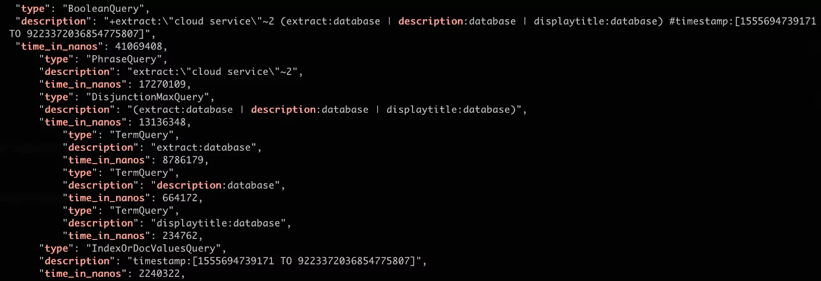
For us, the most important result is the quantity. We can see that the most costly search was the phrase query. This makes sense because it searches for the specific sequence of terms in all of the relevant docs. (Note: we have also added the slop parameter of 2 which allows for up to two other terms to appear between the queried terms).
Next let’s breakdown some of these queries. For instance, let’s examine the match phrase query:
echo "$profile_result" | jq '.profile.shards[].searches[].query[].children[0].breakdown'
The output becomes progressively more detailed:
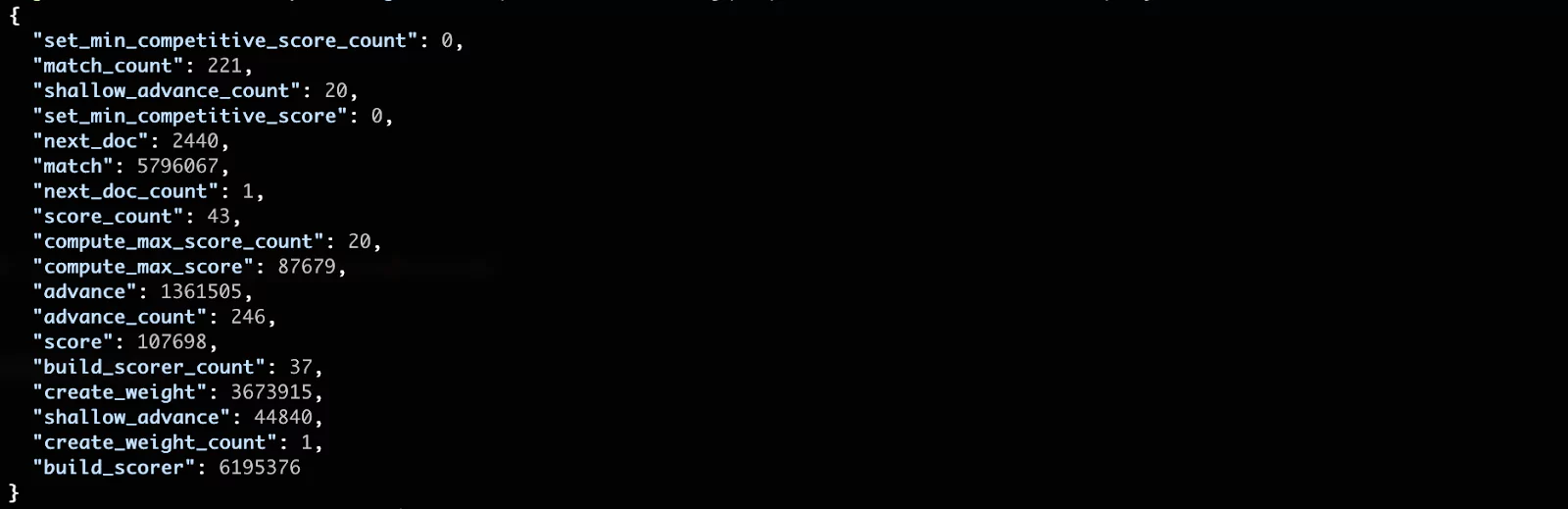
You can see that the most costly phase seems to be the build_scorer, which is a method for scoring the documents. The matching of documents (match phase) follows close after. In most cases these low level results are not the most meaningful for us. This is because we are running in a “lab” environment with a small amount of data. These numbers become much more significant in a production environment.
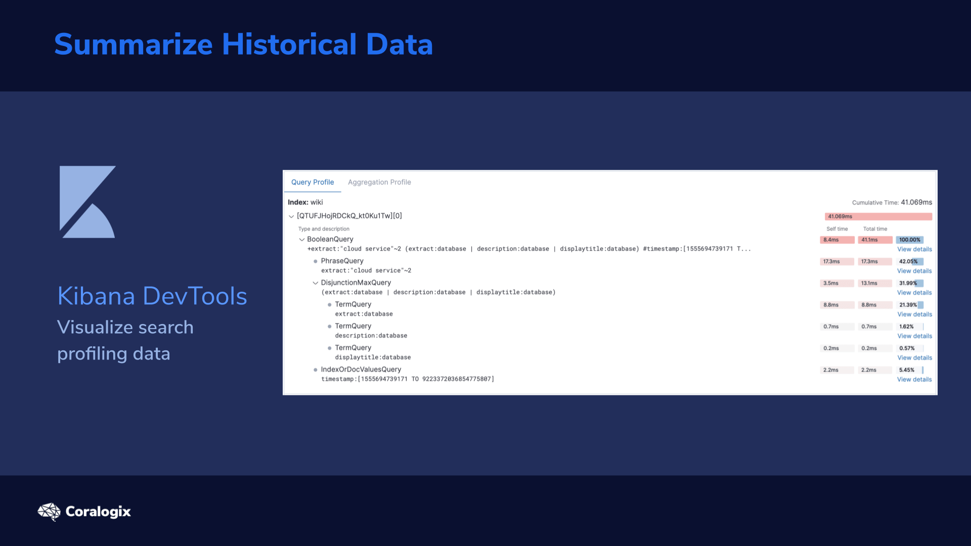
Profiling – Kibana
To see everything we have discussed but in a nice visualized format, you can try the related section in Kibana Dev Tools.
You have two options for using this feature:
- Copy a specific query (or an aggregation) into the text editor area and execute the profiling. (Note: don’t forget to limit the execution to a single index; otherwise the profiler will run on all).
- Or, if you have a few pre-captured profiling results you can copy these into the text editor as well; the profiler will recognize that it is already a profiling output and visualize the results for you.
Try the first option with a new query so you can practice your new skills.
For the second option, you can echo our current payload, copy it from the command line, and paste it into the Kibana profiler.
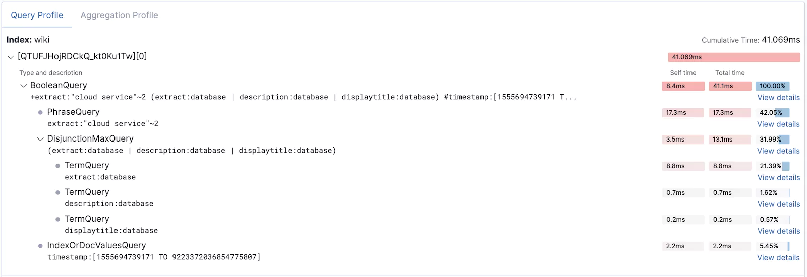
echo "$profile_result" | jq
After execution, you will see the same metrics as before but in a more visually appealing way. You can use the View details link to drill down to a breakdown of a specific query. On the second tab you will find details for any aggregation profiled.
At this point, you now know how to capture sluggish queries in your cluster with the Slow Log and how to use the Profile API and Kibana profiler to dig deeper into your query execution times to improve search performance for your end users.
Learn More
- More details on the breakdowns and other details in the Profile API docs.
- You can also start learning more about Apache Lucene.
This feature is not part of the open-source license but is free to use