Running ELK on Kubernetes with ECK – Part 1

More and more employers are looking for people experienced in building and running Kubernetes-based systems, so it’s a great time to start learning how to take advantage of the new technology. Elasticsearch consists of multiple nodes working together, and Kubernetes can automate the process of creating these nodes and taking care of the infrastructure for us, so running ELK on Kubernetes can be a good options in many scenarios.

We’ll start this with an overview of Kubernetes and how it works behind the scenes. Then, armed with that knowledge, we’ll try some practical hands-on exercises to get our hands dirty and see how we can build and run Elastic Cloud on Kubernetes, or ECK for short.

What we’ll cover:

  • Fundamental Kubernetes concepts
  • Use Vagrant to create a Kubernetes cluster with one master node and two worker nodes
  • Create Elasticsearch clusters on Kubernetes
  • Extract a password from Kubernetes secrets
  • Publicly expose services running on Kubernetes Pods to the Internet, when needed.
  • How to install Kibana
  • Inspect Pod logs
  • Install the Kubernetes Web UI (i.e. Dashboard)
  • Install plugins on an Elasticsearch node running in a Kubernetes container
System Requirements: Before proceeding further, we recommend a system with at least 12GB of RAM, 8 CPU cores, and a fast internet connection. If your computer doesn’t meet the requirements, just use a VPS (virtual private server) provider. Google Cloud is one service that meets the requirements, as it supports nested virtualization on Ubuntu (VirtualBox works on their servers).

There’s a trend, lately, to run everything in isolated little boxes, either virtual machines or containers. There are many reasons for doing this so we won’t get into it here, but if you’re interested, you can read Google’s motivation for using containers

Let’s just say that containers make some aspects easier for us, especially in large-scale operations.

Managing one, two, or three containers is no big deal and we can usually do it manually. But when we have to deal with tens or hundreds of them, we need some help. 

This is where Kubernetes comes in.

What is Kubernetes?

By way of analogy, if containers are the workers in a company, then Kubernetes would be the manager, supervising everything that’s happening and taking appropriate measures to keep everything running smoothly.

After we define a plan of action, Kubernetes does the heavy lifting to fulfill our requirements.

Examples of what you can do with K8s:

  • Launch hundreds of containers, or whatever number needed with much less effort
  • Set up ways that containers can communicate with each other (i.e. networking)
  • Automatically scale up or down. When demand is high, create more containers, even on multiple physical servers, so that the stress of the high demand is distributed across multiple machines, making it easier to process. As soon as demand goes down, it can remove unneeded containers, as well as the nodes that were hosting them (if they’re sitting idle).
  • If there are a ton of requests coming in, Kubernetes can load balance and evenly distribute the workload to multiple containers and nodes.
  • Containers are carefully monitored with health checks, according to user-defined specifications. If one stops working, Kubernetes can restart it, create a new one as a replacement, or kill it entirely. If a physical machine running containers fails, those containers can be moved to another physical machine that’s still working correctly.

Kubernetes Cluster Structure
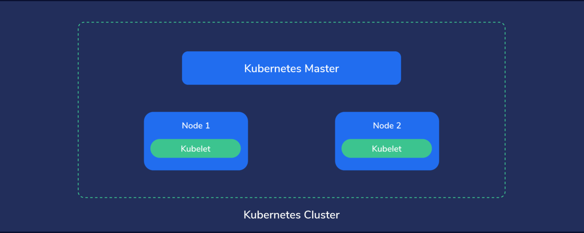
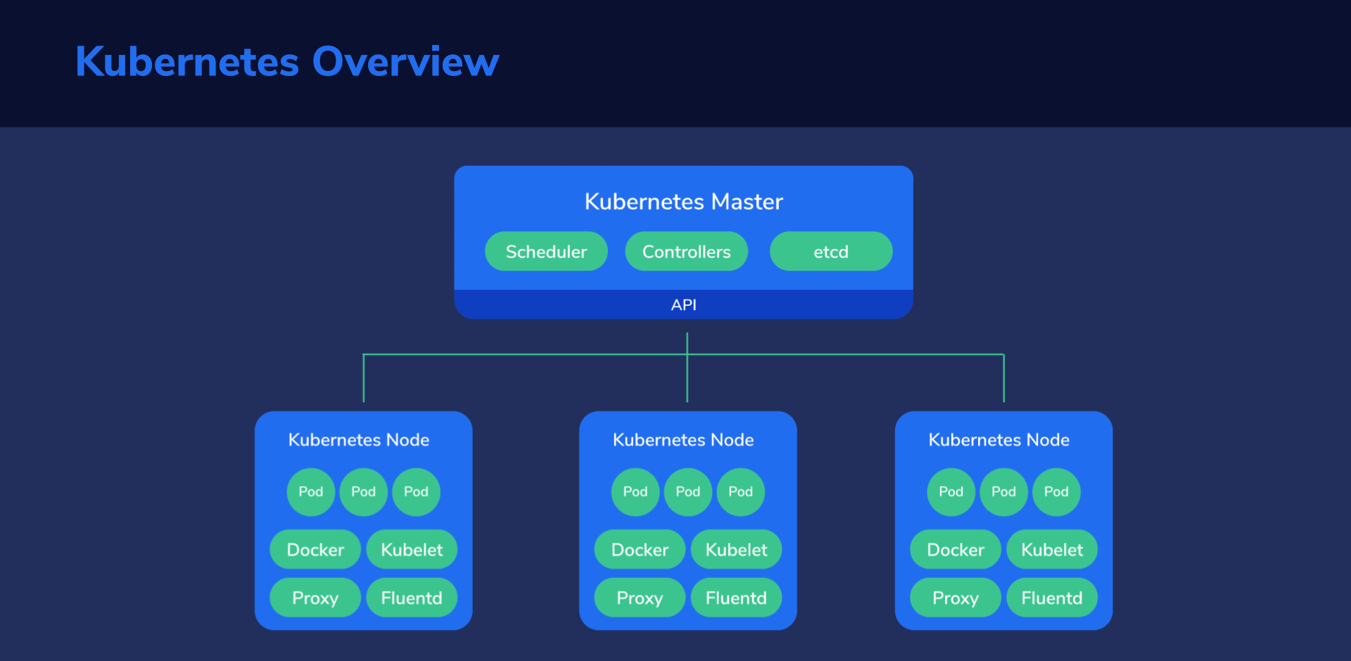
Let’s analyze the structure from the top down to get a good handle on things before diving into the hands-on section.

First, Kubernetes must run on computers of some kind. It might end up being on dedicated servers, virtual private servers, or virtual machines hosted by a capable server. 

Multiple such machines running Kubernetes components form a Kubernetes cluster, which is considered the whole universe of Kubernetes, because everything, from containers to data, to monitoring systems and networking exists here. 

In this little universe, there has to be a central point of command, like the “brains” of Kubernetes. We call this the master node. This node assumes control of the other nodes, sometimes also called worker nodes. The master node manages the worker nodes, while these, in turn, run the containers and do the actual work of hosting our applications, services, processing data, and so on.

Master Node

Basically, we’re the master of our master node, and it, in turn, is the master of every other node.

We instruct our master node about what state we want to achieve which then proceeds to take the necessary steps to fulfill our demands. 

Simply put, it automates our plan of action and tries to keep the system state within set parameters, at all times.

Nodes (or Worker Nodes)

The Nodes are like the “worker bees” of a Kubernetes cluster and provide the physical resources, such as CPU, storage space, memory, to run our containers.

Basic Kubernetes Concepts

Up until this point, we kept things simple and just peaked at the high-level structure of a Kubernetes cluster. So now let’s zoom in and take a closer look at the internal structure so we better understand what we’re about to get our hands dirty with.

Pods

Pods are like the worker ants of Kubernetes – the smallest units of execution. They are where applications run and do their actual work, processing data. A Pod has its own storage resources, and its own IP address and runs a container, or sometimes, multiple containers grouped together as a single entity.

Services

Pods can appear and disappear at any moment, each time with a different IP address. It would be quite hard to send requests to Pods since they’re basically a moving target. To get around this, we use Kubernetes Services.

A K8s Service is like a front door to a group of Pods. The service gets its own IP address. When a request is sent to this IP address, the service then intelligently redirects it to the appropriate Pod. We can see how this approach provides a fixed location that we can reach. It can also be used as a mechanism for things like load balancing. The service can decide how to evenly distribute all incoming requests to appropriate Pods.

Namespaces

Physical clusters can be divided into multiple virtual clusters, called namespaces. We might use these for a scenario in which two different development teams need access to one Kubernetes cluster. 

With separate namespaces, we don’t need to worry if one team screws up the other team’s namespace since they’re logically isolated from one another.

Deployments

In deployments, we describe a state that we want to achieve. Kubernetes then proceeds to work its magic to achieve that state. 

Deployments enable:

  • Quick updates – all Pods can gradually be updated, one-by-one, by the Deployment Controller. This gets rid of having to manually update each Pod. A tedious process no one enjoys.
  • Maintain the health of our structure – if a Pod crashes or misbehaves, the controller can replace it with a new one that works.
  • Recover Pods from failing nodes – if a node should go down, the controller can quickly launch working Pods in another, functioning node.
  • Automatically scale up and down based on the CPU utilization of Pods.
  • Rollback changes that created issues. We’ve all been there 🙂

Labels and Selectors

First, things like Pods, services, namespaces, volumes, and the like, are called “objects”. We can apply labels to objects. Labels help us by grouping and organizing subsets of these objects that we need to work with. 

The way Labels are constructed is with key/value pairs. Consider these examples:

app:nginx

site:example.com

Applied to specific Pods, it can easily help us identify and select those that are running the Nginx web server and are hosting a specific website.

And finally, with a selector, we can match the subset of objects we intend to work with. For example, a selector like

app = nginx

site = example.com

This would match all the Pods running Nginx and hosting “example.com”.

Ingress

In a similar way that Kubernetes Services sit in front of Pods to redirect requests, Ingress sits in front of Services to load balance between different Services using SSL/TLS to encrypt web traffic or using name-based hosting. 

Let’s take an example to explain name-based hosting. Say there are two different domain names, for example, “a.example.com” and “b.example.com” pointing to the same ingress IP address. Ingress can be made to route requests coming from “a.example.com” to service A and requests from “b.example.com” to service B.

Stateful Sets

Deployments assume that applications in Kubernetes are stateless, that is, they start and finish their job and can then be terminated at any time – with no state being preserved. 

However, we’ll need to deal with Elasticsearch, which needs a stateful approach. 

Kubernetes has a mechanism for this called StatefulSets. Pods are assigned persistent identifiers, which makes it possible to do things like:

  • Preserve access to the same volume, even if the Pod is restarted or moved to another node.
  • Assign persistent network identifiers, even if Pods are moved to other nodes.
  • Start Pods in a certain order, which is useful in scenarios where Pod2 depends on Pod1 so, obviously, Pod1 would need to start first, every time.
  • Rolling updates in a specific order.

Persistent Volumes

A persistent volume is simply storage space that has been made available to the Kubernetes cluster. This storage space can be provided from the local hardware, or from cloud storage solutions.

When a Pod is deleted, its associated volume data is also deleted. As the name suggests, persistent volumes preserve their data, even after a Pod that was using it disappears. Besides keeping data around, it also allows multiple Pods to share the same data.

Before a Pod can use a persistent volume, though,  it needs to make a Persistent Volume Claim on it.

Headless Service

We previously saw how a Service sits in front of a group of Pods, acting as a middleman, redirecting incoming requests to a dynamically chosen Pod. But this also hides the Pods from the requester, since it can only “talk” with the Service’s IP address. 

If we remove this IP, however, we get what’s called a Headless Service. At that point, the requester could bypass the middle man and communicate directly with one of the Pods. That’s because their IP addresses are now made available to the outside world.

This type of service is often used with Stateful Sets.

Kubectl

Now, we need a way to interact with our entire Kubernetes cluster. The kubectl command allows us to enter commands to get kubectl to do what we need. It then interacts with the Kubernetes API, and all of the other components, to execute our desired actions.

Let’s look at a few simple commands. 

For example, to check the cluster information, we’d would enter:

kubectl cluster-info

If we wanted to list all nodes in the cluster, we’d enter:

kubectl get nodes

We’ll take a look at many more examples in our hands-on exercises.

Operators

Some operations can be complex. For example, upgrading an application might require a large number of steps, verifications, and decisions on how to act if something goes wrong. This might be easy to with one installation, but what if we have 1000 to worry about? 

In Kubernetes, hundreds, thousands, or more containers might be running at any given point. If we would have to manually do a similar operation on all of them, it’s why we’d want to automate that.

Enter Operators. We can think of them as a sort of “software operators,” replacing the need for human operators. These are written specifically for an application, to help us, as service owners, to automate tasks.

Operators can deploy and run the many containers and applications we need, react to failures and try to recover from them, automatically backup data, and so on. This essentially lets us extend Kubernetes beyond its out-of-the-box capabilities without modifying the actual Kubernetes code.

Custom Resources

Since Kubernetes is modular by design, we can extend the API’s basic functionality. For example, the default installation might not have appropriate mechanisms to deal efficiently with our specific application and needs. By registering a new Custom Resource Definition, we can add the functionality we need, custom-tailored for our specific application. In our exercises, we’ll explore how to add Custom Resource Definitions for various Elasticsearch applications.

Hands-On Exercises

Basic Setup

Ok, now the fun begins. We’ll start by creating virtual machines that will be added as nodes to our Cluster. We will use VirtualBox to make it simpler.

1. Installing VirtualBox

1.1 Installing VirtualBox on Windows

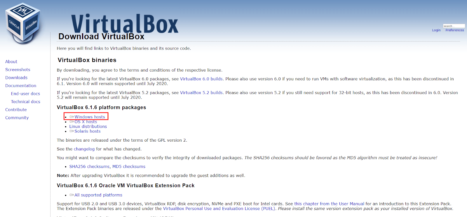
Let’s go to the download page: https://www.virtualbox.org/wiki/Downloads and click on “Windows Hosts”.
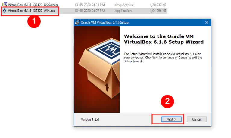
We can then open the setup file we just downloaded and click “Next” in the installation wizard, keeping the default options selected.
After finishing with the installation, it’s a good idea to check if everything works correctly by opening up VirtualBox, either from the shortcut added to the desktop, or the Start Menu.
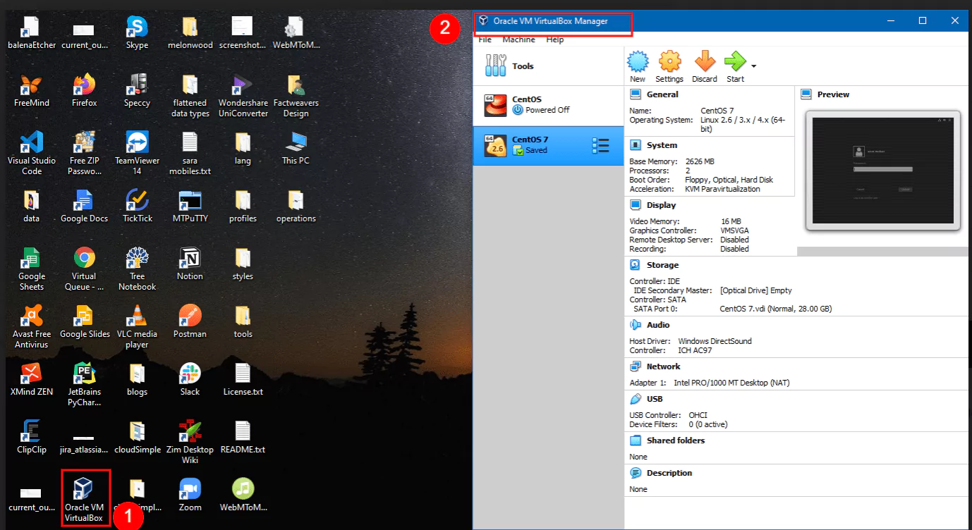
If everything seems to be in order, we can close the program and continue with the Vagrant setup.

1.2 Installing VirtualBox on Ubuntu

First, we need to make sure that the Ubuntu Multiverse repository is enabled.

Afterward, we install VirtualBox with the next command:

sudo apt-get update && sudo apt-get install virtualbox-qt

Let’s try to run VirtualBox to ensure the install was successful:

virtualbox
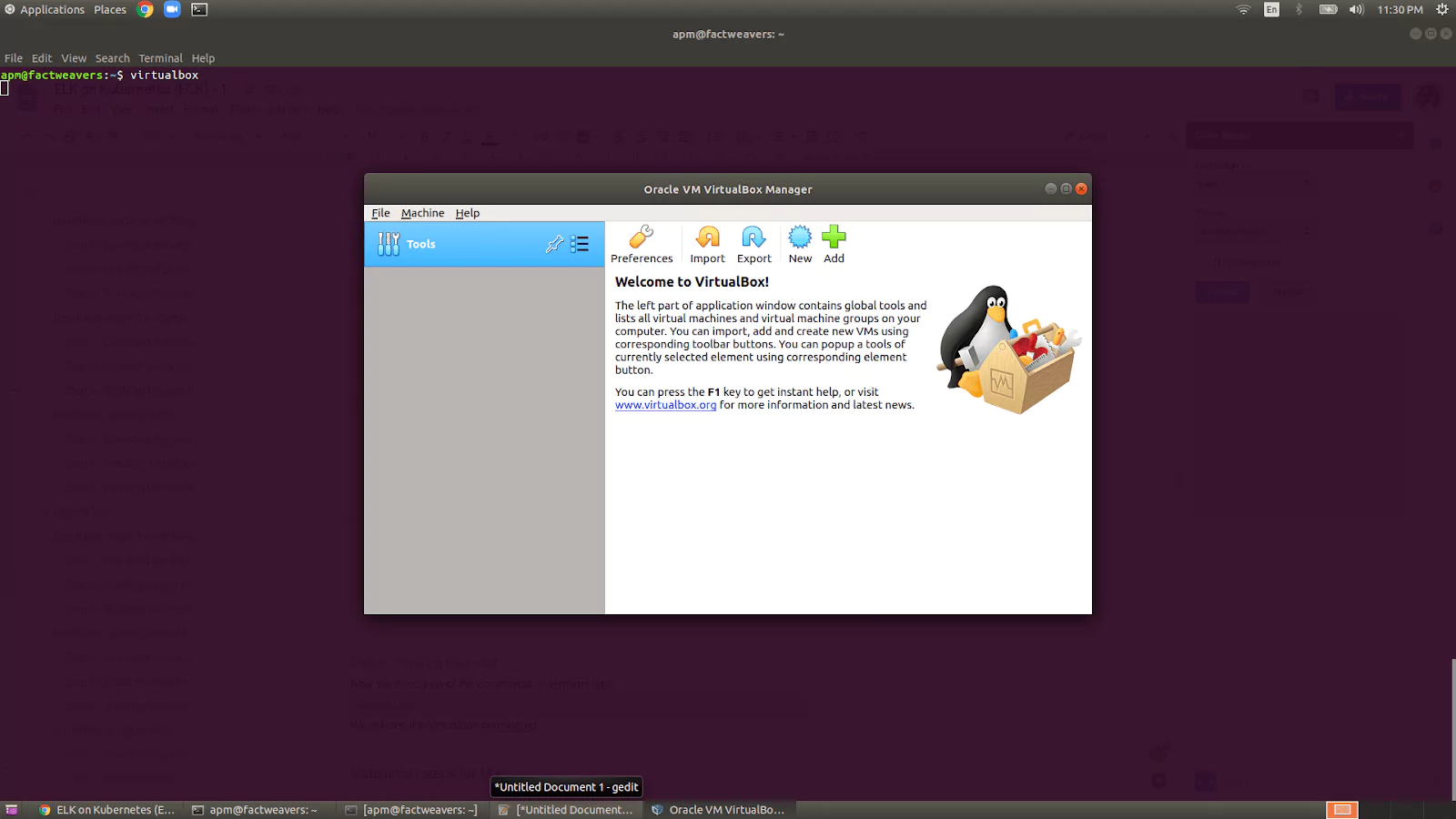
Once the app opens up, we can close it and continue with Vagrant.

1.3 Installing VirtualBox on macOS

Let’s download the setup file from https://www.virtualbox.org/wiki/Downloads and click on “OS X hosts.”
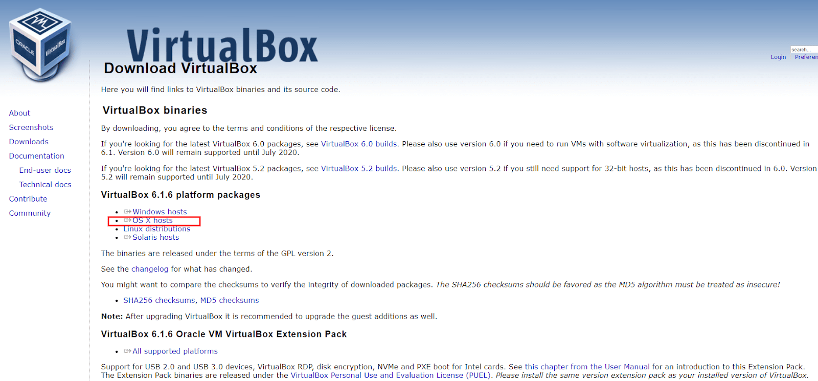
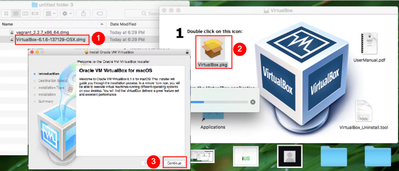
We can now open the DMG file, execute the PKG inside and run the installer. We keep the default options selected and continue with the steps in the install wizard.
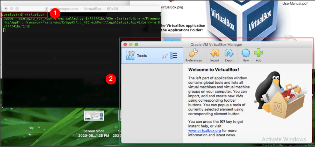
Let’s open up the terminal and check if the install was successful.

virtualbox

If the application opens up and everything seems to be in order, we can continue with the Vagrant setup.
2. Installing Vagrant

It would be pretty time-consuming to set up each virtual machine for use with Kubernetes. But we will use Vagrant, a tool that automates this process, making our work much easier.

2.1 Installing Vagrant on Windows

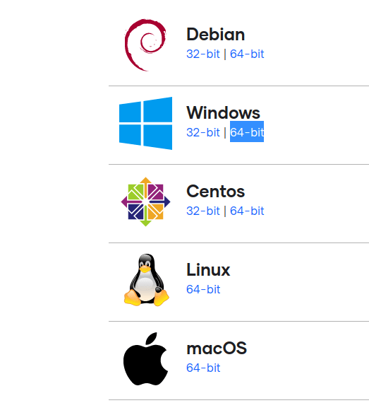
Installing on Windows is easy. We just need to visit the following address, https://www.vagrantup.com/downloads.html, and click on the appropriate link for the Windows platform. Nowadays, it’s almost guaranteed that everyone would need the 64-bit executable. Only download the 32-bit program if you’re certain your machine has an older, 32-bit processor.
Now we just need to follow the steps in the install wizard, keeping the default options selected.
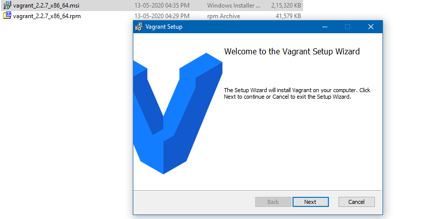
If at the end of the setup you’re prompted to restart your computer, please do so, to make sure all components are configured correctly.

Let’s see if the “vagrant” command is available. Click on the Start Menu, type “cmd” and open up “Command Prompt”. Next, type:

vagrant --version

If the program version is displayed, we can move on to the next section and provision our Kubernetes cluster.

2.2 Installing Vagrant on Ubuntu

First, we need to make sure that the Ubuntu Universe repository is enabled.

If that’s enabled, installing Vagrant is as simple as running the following command:

sudo apt-get update && sudo apt-get install vagrant

Finally, let’s double-check that the program was successfully installed, with:

vagrant --version

2.3 Installing Vagrant on macOS

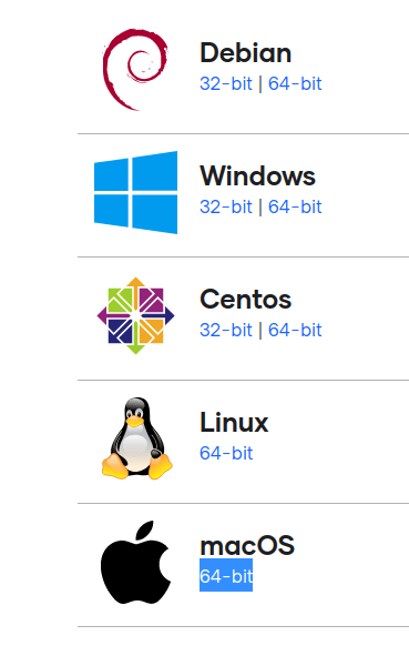
Let’s first download the setup file from https://www.vagrantup.com/downloads.html, which, at the time of this writing, would be found at the bottom of the page, next to the macOS icon.
Once the download is finished, let’s open up the DMG file, execute the PKG inside, and go through the steps of the install wizard, leaving the default selections as they are.
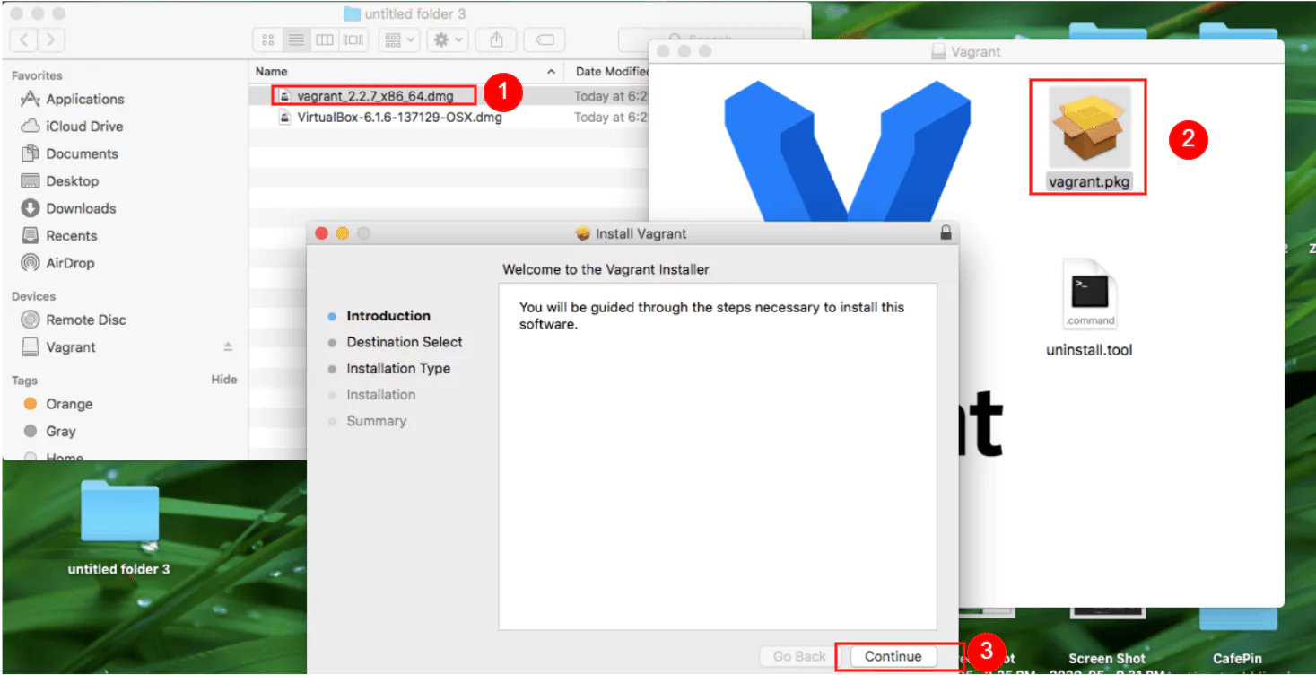
Once the install is complete, we will be presented with this window.
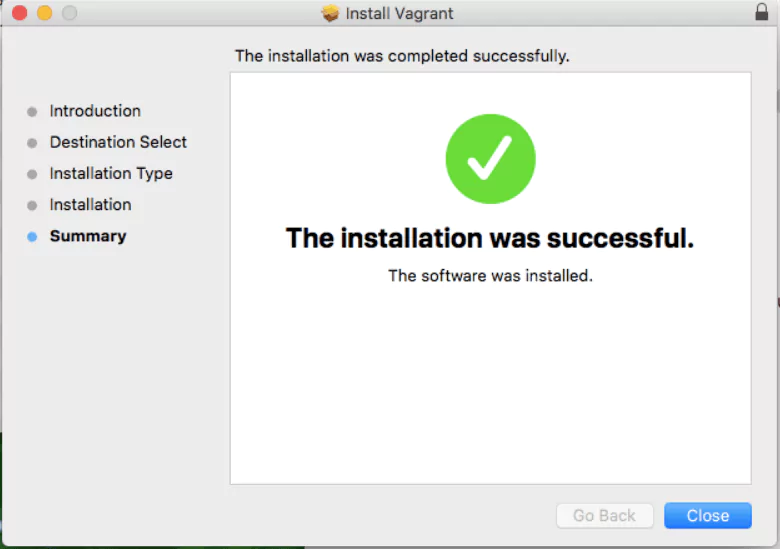
But we can double-check if Vagrant is fully set up by opening up the terminal and typing the next command:

vagrant --version

Provisioning the Kubernetes Cluster 

Vagrant will interact with the VirtualBox API to create and set up the required virtual machines for our cluster. Here’s a quick overview of the workflow.
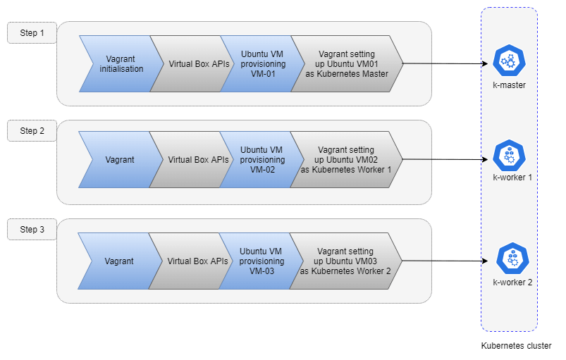
Once Vagrant finishes the job, we will end up with three virtual machines. One machine will be the master node and the other two will be worker nodes.

Let’s first download the files that we will use with Vagrant, from https://github.com/coralogix-resources/elastic-cloud-on-kubernetes-webinar/raw/master/k8s_ubuntu.zip

Credit for files: https://bitbucket.org/exxsyseng/k8s_ubuntu/src/master/

Next, we have to extract the directory “k8s_ubuntu” from this ZIP file.

Now let’s continue, by entering the directory we just unzipped. You’ll need to adapt the next command to point to the location where you extracted your files. 

For example, on Windows, if you extracted the directory to your Desktop, the next command would be “cd Desktopk8s_ubuntu”. 

On Linux, if you extracted to your Downloads directory, the command would be “cd Downloads/k8s_ubuntu”.

cd k8s_ubuntu

We’ll need to be “inside” this directory when we run a subsequent “vagrant up” command.

Let’s take a look at the files within. On Windows, enter:

dir

On Linux/macOS, enter:

ls -lh

The output will look something like this:
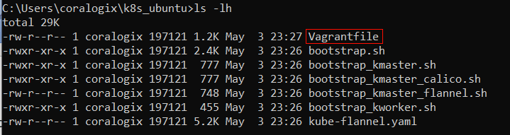
We can see a file named “Vagrantfile”. This is where the main instructions exist, telling Vagrant how it should provision our virtual machines.

Let’s open the file, since we need to edit it:
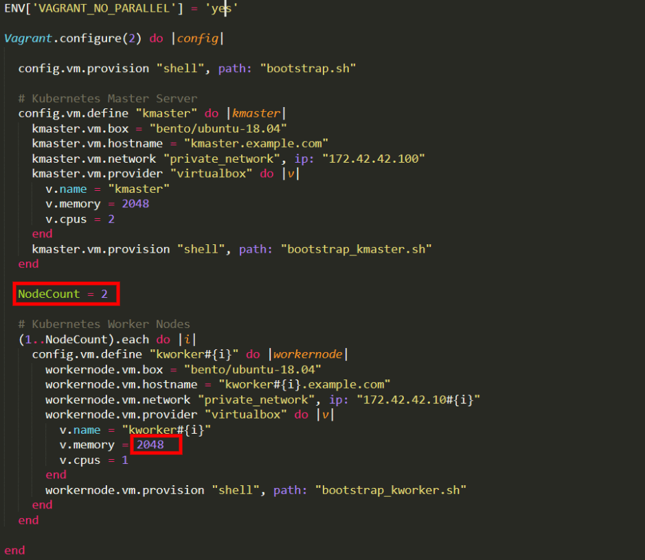
Note: In case you’re running an older version of Windows, we recommend you edit in WordPad instead of Notepad. Older versions of Notepad have trouble interpreting EOL (end of line) characters in this file, making the text hard to read since lines wouldn’t properly be separated.

Look for the text “v.memory” found under the “Kubernetes Worker Nodes” section. We’ll assign this variable a value of 4096, to ensure that each Worker Node gets 4 GB of RAM because Elasticsearch requires at least this amount to function properly with the 4 nodes we will add later on. We’ll also change “v.cpus” and assign it a value of 2 instead of 1.

After we save our edited file, we can finally run Vagrant:

vagrant up

Now, this might take a while since there’re quite a few things that need to be downloaded and set up. We’ll be able to follow its progress in the output and we may get a few prompts to accept some changes.

When the job is done, we can SSH into the master node by typing:

vagrant ssh kmaster
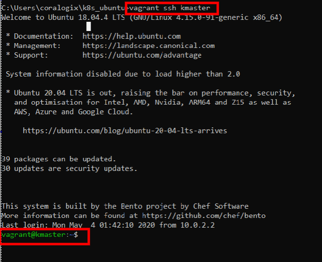
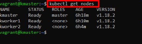
Let’s check if Kubernetes is up and running:

kubectl get nodes

This will list the nodes that make up this cluster:
Pretty awesome! We are well on our way to implementing the ELK stack on Kubernetes. So far, we’ve created our Kubernetes cluster and just barely scratched the surface of what we can do with such automation tools. 

Stay tuned for more about Running ELK on Kubernetes with the rest of the series!

Part 2 – Coming December 22nd, 2020

Part 3 – Coming December 29th, 2020

A Crash Course in Kubernetes Monitoring

Kubernetes log monitoring can be complex. To do it successfully requires several components to be monitored simultaneously. First, it’s important to understand what those components are, which metrics should be monitored and what tools are available to do so.

In this post, we’ll take a close look at everything you need to know to get started with monitoring your Kubernetes-based system.

Monitoring Kubernetes Clusters vs. Kubernetes Pods

Monitoring Kubernetes Clusters

When monitoring the cluster, a full view across all areas is obtained, giving a good impression of the health of all pods, nodes, and apps.

Key areas to monitor at the cluster level include:

  • Node load: Tracking the load on each node is integral to monitoring efficiency. Some nodes are used more than others. Rebalancing the load distribution is key to keeping workloads fluid and effective. This can be done via DaemonSets.
  • Unsuccessful pods: Pods fail and abort. This is a normal part of Kubernetes processes. When a pod that should be working at a more efficient level or is inactive, it is essential to investigate the reason behind the anomalies in pod failures.
  • Cluster usage: Monitoring cluster infrastructure allows adjustment of the number of nodes in use and the allocation of resources to power workloads efficiently. The visibility of resources being distributed allows scaling up or down and avoids the costs of additional infrastructure. It is important to set a container’s memory and CPU usage limit accordingly.

Monitoring Kubernetes Pods

Cluster monitoring provides a global view of the Kubernetes environment, but collecting data from individual pods is also essential. It reveals the health of individual pods and the workloads they are hosting, providing a clearer picture of pod performance at a granular level, beyond the cluster. 

Key areas to monitor at the cluster level include:

  • Total pod instances: There needs to be enough instances of a pod to ensure high availability. This way hosting bandwidth is not wasted, however consideration is needed to not run ‘too many extra’ pod instances.
  • Actual pod instances: Monitoring the number of instances for each pod that’s running versus what is expected to be running will reveal how to redistribute resources to achieve the desired state in terms of pods instances. ReplicaSets could be misconfigured with varying metrics, so it’s important to analyze these regularly.
  • Pod deployment: Monitoring pods deployment allows to view any misconfigurations that might be diminishing the availability of pods. It’s critical to monitor how resources distribute to nodes.

Important Metrics for Kubernetes Monitoring

To gain a higher visibility into a Kubernetes installation, there are several metrics that will provide valuable insight into how the apps are running.

Common metrics

These are metrics collected from the Kubernetes code, written in Golang. They allow understanding of performance in the platform at a cellular level and display the state of what is happening in the GoLang processes.

Node metrics –

Monitoring the standard metrics from the operating systems that power Kubernetes nodes provides insight into the health of each node.

Each Kubernetes Node has a finite capacity of memory and CPU and that can be utilized by the running pods, so these two metrics need to be monitored carefully. Other common node metrics to monitor include CPU load, memory consumption, filesystem activity and usage and network activity.

One approach to monitoring all cluster nodes is to create a special kind of Kubernetes pod called DaemonSets. Kubernetes ensures that every node created has a copy of the DaemonSet pod, which virtually enables one deployment to watch each machine in the cluster. As nodes are destroyed, the pod is also terminated.

Kubelet metrics –

To ensure the Control Plane is communicating efficiently with each individual node that a Kubelet runs on, it is recommended to monitor the Kubelet agent regularly. Beyond the common GoLang common metrics described above, Kubelet exposes some internals about its actions that are useful to track as well.

Controller manager metrics –

To ensure that workloads are orchestrated effectively, monitor the requests that the Controller is making to external APIs. This is critical in cloud-based Kubernetes deployments.

Scheduler metrics

To identify and prevent delays, monitor latency in the scheduler. This will ensure Kubernetes is deploying pods smoothly and on time.

The main responsibility of the scheduler is to choose which nodes to start newly launched pods on, based on resource requests and other conditions.

The scheduler logs are not very helpful on their own. Most of the scheduling decisions are available as Kubernetes events, which can be logged easily in a vendor-independent way, thus are the recommended source for troubleshooting. The scheduler logs might be needed in the rare case when the scheduler is not functioning, but a kubectl logs call is usually sufficient.

etcd metrics –

etcd stores all the configuration data for Kubernetes. etcd metrics will provide essential visibility into the condition of the cluster.

Container metrics –

Looking specifically into individual containers will allow monitoring of exact resource consumption rather than more general Kubernetes metrics. CAdvisor analyzes resource usage happening inside containers.

API Server metrics –

The Kubernetes API server is the interface to all the capabilities that Kubernetes provides. The API server controls all the operations that Kubernetes can perform. Monitoring this critical component is vital to ensure a smooth running cluster.

The API server metrics are grouped into a major categories:

  • Request Rates and Latencies
  • Performance of controller work queues
  • etcd helper cache work queues and cache performance
  • General process status (File Descriptors/Memory/CPU Seconds)
  • Golang status (GC/Memory/Threads)

kube-state-metrics –

kube-state-metrics is a service that makes cluster state information easily consumable. Where the Metrics Server exposes metrics on resource usage by pods and nodes, kube-state-metrics listens to the Control Plane API server for data on the overall status of Kubernetes objects (nodes, pods, Deployments, etc) as well as the resource limits and allocations for those objects. It then generates metrics from that data that are available through the Metrics API.

kube-state-metrics is an optional add-on. It is very easy to use and exports the metrics through an HTTP endpoint in a plain text format. They were designed to be easily consumed / scraped by open source tools like Prometheus.

In Kubernetes, the user can fetch system-level metrics from various out of the box tools like cAdvisor, Metrics Server, and Kubernetes API Server. It is also possible to fetch application level metrics from integrations like kube-state-metrics and Prometheus Node Exporter.

Prometheus scrapes metrics from instrumented jobs, either directly or via an intermediary push gateway for short-lived jobs. It locally stores all scraped samples and runs rules over this data to either aggregate and record new time series from existing data or generate alerts. Grafana or other API tools can be used to visualize the collected data.

Prometheus, Grafana and Alertmanager

One of the most popular Kubernetes monitoring solutions is the open-source Prometheus, Grafana and Alertmanager stack, deployed alongside kube-state-metrics and node_exporter to expose cluster-level Kubernetes object metrics as well as machine-level metrics like CPU and memory usage.

What is Prometheus?

Prometheus is a pull-based tool used specifically for containerized environments like Kubernetes. It is primarily focused on the metrics space and is more suited for operational monitoring. Exposing and scraping prometheus metrics is straightforward, and they are human readable, in a self-explanatory format. The metrics are published using a standard HTTP transport and can be checked using a web browser. 

Apart from application metrics, Prometheus can collect metrics related to:

  • Node exporter, for the classical host-related metrics: cpu, mem, network, etc.
  • Kube-state-metrics for orchestration and cluster level metrics: deployments, pod metrics, resource reservation, etc.
  • Kube-system metrics from internal components: kubelet, etcd, scheduler, etc.

Prometheus can configure rules to trigger alerts using PromQL, Alertmanager will be in charge of managing alert notification, grouping, inhibition, etc.

Using Prometheus with Alertmanager and Grafana

PromQL (Prometheus Query Language) lets the user choose time-series data to aggregate and then view the results as tabular data or graphs in the Prometheus expression browser. Results can also be consumed by the external system via an API.

How does Alertmanager fit in? The Alertmanager component configures the receivers, gateways to deliver alert notifications. It handles alerts sent by client applications such as the Prometheus server and takes care of deduplicating, grouping, and routing them to the correct receiver integration such as email, PagerDuty or OpsGenie. It also takes care of silencing and inhibition of alerts.

Grafana can pull metrics from any number of Prometheus servers and display panels and dashboards. It also has the added ability to register multiple different backends as a datasource and render them all out on the same dashboard. This makes Grafana an outstanding choice for monitoring dashboards.

Useful Log Data for Troubleshooting

Logs are useful to examine when a problem is revealed by metrics. They give exact and invaluable information which provides more details than metrics. There are many options for logging in most of Kubernetes’ components. Applications also generate log data.

Digging deeper into the cluster requires logging into the relevant machines.

The locations of the relevant log files are:

  • Master

/var/log/kube-apiserver.log – API Server, responsible for serving the API

/var/log/kube-scheduler.log – Scheduler, responsible for making scheduling decisions

/var/log/kube-controller-manager.log – Controller that manages replication controllers

  • Worker nodes

/var/log/kubelet.log – Kubelet, responsible for running containers on the node

/var/log/kube-proxy.log – Kube Proxy, responsible for service load balancing

  • etcd logs

etcd uses the Github capnslog library for logging application output categorized into levels.           

A log message’s level is determined according to these conventions:

  • Error: Data has been lost, a request has failed for a bad reason, or a required resource has been lost.
  • Warning: Temporary conditions that may cause errors, but may work fine.
  • Notice: Normal, but important (uncommon) log information.
  • Info: Normal, working log information, everything is fine, but helpful notices for auditing or common operations.
  • Debug: Everything is still fine, but even common operations may be logged and less helpful but more quantity of notices.

kubectl

When it comes to troubleshooting the Kubernetes cluster and the applications running on it, understanding and using logs are crucial. Like most systems, Kubernetes maintains thorough logs of activities happening in the cluster and applications, which highlight the root causes of any failures.

Logs in Kubernetes can give an insight into resources such as nodes, pods, containers, deployments and replica sets. This insight allows the observation of the interactions between those resources and see the effects that one action has on another. Generally, logs in the Kubernetes ecosystem can be divided into the cluster level (logs outputted by components such as the kubelet, the API server, the scheduler) and the application level (logs generated by pods and containers).

Use the following syntax to run kubectl commands from your terminal window:

kubectl [command] [TYPE] [NAME] [flags]

Where:

  • command: the operation to perform on one or more resources, i.e. create, get, describe, delete.
  • TYPE: the resource type.
  • NAME: the name of the resource.
  • flags: optional flags.

Examples:

kubectl get pod pod1    # Lists resources of the pod ‘pod1’
kubectl logs pod1    # Returns snapshot logs from the pod ‘pod1’ 

Kubernetes Events

Since Kubernetes Events capture all the events and resource state changes happening in your cluster, they allow past activities to be analyzed in your cluster. They are objects that display what is happening inside a cluster, such as the decisions made by the scheduler or why some pods were evicted from the node. They are the first thing to inspect for application and infrastructure operations when something is not working as expected.

Unfortunately, Kubernetes events are limited in the following ways:

  • Kubernetes Events can generally only be accessed using kubectl.
  • The default retention period of kubernetes events is one hour.
  • The retention period can be increased but this can cause issues with the cluster’s key-value store.
  • There is no way to visualize these events.

To address these issues, open source tools like Kubewatch, Eventrouter and Event-exporter have been developed.

Summary

Kubernetes monitoring is performed to maintain the health and availability of containerized applications built on Kubernetes. When you are creating the monitoring strategy for Kubernetes-based systems, it’s important to keep in mind the top metrics to monitor along with the various monitoring tools discussed in this article.

Running Elasticsearch, Logstash, and Kibana on Kubernetes with Helm

Kubernetes monitoring (or “K8s”) is an open-source container orchestration tool developed by Google. In this tutorial, we will be leveraging the power of Kubernetes to look at how we can overcome some of the operational challenges of working with the Elastic Stack.

Since Elasticsearch (a core component of the Elastic Stack) is comprised of a cluster of nodes, it can be difficult to roll out updates, monitor and maintain nodes, and handle failovers. With Kubernetes, we can cover all of these points using built in features: the setup can be configured through code-based files (using a technology known as Helm), and the command line interface can be used to perform updates and rollbacks of the stack. Kubernetes also provides powerful and automatic monitoring capabilities that allows it to notify when failures occur and attempt to automatically recover from them.

This tutorial will walk through the setup from start to finish. It has been designed for working on a Mac, but the same can also be achieved on Windows and Linux (albeit with potential variation in commands and installation).

Prerequisites

Before we begin, there are a few things that you will need to make sure you have installed, and some more that we recommend you read up on. You can begin by ensuring the following applications have been installed on your local system.

While those applications are being installed, it is recommended you take the time to read through the following links to ensure you have a basic understanding before proceeding with this tutorial.

Let’s get started

As part of this tutorial, we will cover 2 approaches to cover the same problem. We will start by manually deploying individual components to Kubernetes and configuring them to achieve our desired setup. This will give us a good understanding of how everything works. Once this has been accomplished, we will then look at using Helm Charts. These will allow us to achieve the same setup but using YAML files that will define our configuration and can be deployed to Kubernetes with a single command.

The manual approach

Deploying Elasticsearch

First up, we need to deploy an Elasticsearch instance into our cluster. Normally, Elasticsearch would require 3 nodes to run within its own cluster. However, since we are using Minikube to act as a development environment, we will configure Elasticsearch to run in single node mode so that it can run on our single simulated Kubernetes node within Minikube.

So, from the terminal, enter the following command to deploy Elasticsearch into our cluster.

$ kubectl create deployment es-manual --image elasticsearch:7.8.0

[Output]
deployment.apps/es-manual created

Note: I have used the name “es-manual” here for this deployment, but you can use whatever you like. Just be sure to remember what you have used.

Since we have not specified a full URL for a Docker registry, this command will pull the image from Docker Hub. We have used the image elasticsearch:7.8.0 – this will be the same version we use for Kibana and Logstash as well.

We should now have a Deployment and Pod created. The Deployment will describe what we have deployed and how many instances to deploy. It will also take care of monitoring those instances for failures and will restart them when they fail. The Pod will contain the Elasticsearch instance that we want to run. If you run the following commands, you can see those resources. You will also see that the instance is failing to start and is restarted continuously.

$ kubectl get deployments

[Output]
NAME        READY   UP-TO-DATE   AVAILABLE   AGE
es-manual   1/1     1            1           8s

$ kubectl get pods

[Output]
NAME                        READY   STATUS    RESTARTS   AGE
es-manual-d64d94fbc-dwwgz   1/1     Running   2          40s

Note: If you see a status of ContainerCreating on the Pod, then that is likely because Docker is pulling the image still and this may take a few minutes. Wait until that is complete before proceeding.

For more information on the status of the Deployment or Pod, use the kubectl describe or kubectl logs commands:

$ kubectl describe deployment es-manual
$ kubectl describe pod es-manual-d64d94fbc-dwwgz
$ kubectl logs –f deployments/es-manual

An explanation into these commands is outside of the scope of this tutorial, but you can read more about them in the official documentation: describe and logs.

In this scenario, the reason our Pod is being restarted in an infinite loop is because we need to set the environment variable to tell Elasticsearch to run in single node mode. We are unable to do this at the point of creating a Deployment, so we need to change the variable once the Deployment has been created. Applying this change will cause the Pod created by the Deployment to be terminated, so that another Pod can be created in its place with the new environment variable.

ERROR: [1] bootstrap checks failed
[1]: the default discovery settings are unsuitable for production use; at least one of [discovery.seed_hosts, discovery.seed_providers, cluster.initial_master_nodes] must be configured

The error taken from the deployment logs that describes the reason for the failure.

Unfortunately, the environment variable we need to change has the key “discovery.type”. The kubectl program does not accept “.” characters in the variable key, so we need to edit the Deployment manually in a text editor. By default, VIM will be used, but you can switch out your own editor (see here for instructions on how to do this). So, run the following command and add the following contents into the file:

$ kubectl edit deployment es-manual

apiVersion: apps/v1
kind: Deployment
...
containers:
- name: elasticsearch
env:
- name: discovery.type
value: single-node
image: elasticsearch:7.8.0
imagePullPolicy: IfNotPresent
...

If you now look at the pods, you will see that the old Pod is being or has been terminated, and the new Pod (containing the new environment variable) will be created.

$ kubectl get pods

[Output]
NAME                         READY   STATUS        RESTARTS   AGE
es-manual-7d8bc4cf88-b2qr9   1/1     Running       0           7s
es-manual-d64d94fbc-dwwgz    0/1     Terminating   8           21m

Exposing Elasticsearch

Now that we have Elasticsearch running in our cluster, we need to expose it so that we can connect other services to it. To do this, we will be using the <code>expose command. To briefly explain, this command will allow us to expose our Elasticsearch Deployment resource through a Service that will give us the ability to access our Elasticsearch HTTP API from other resources (namely Logstash and Kibana). Run the following command to expose our Deployment:

$ kubectl expose deployment es-manual --type NodePort --port 9200

[Output]
service/es-manual exposed

This will have created a Kubernetes Service resource that exposes the port 9200 from our Elasticsearch Deployment resource: Elasticsearch’s HTTP port. This port will now be accessible through a port assigned in the cluster. To see this Service and the external port that has been assigned, run the following command:

$ kubectl get services

[Output]
NAME         TYPE        CLUSTER-IP      EXTERNAL-IP   PORT(S)
es-manual    NodePort    10.96.114.186          9200:30445/TCP  
kubernetes   ClusterIP  10.96.0.1               443/TCP

As you can see, our Elasticsearch HTTP port has been mapped to external port 30445. Since we are running through Minikube, the external port will be for that virtual machine, so we will use the Minikube IP address and external port to check that our setup is working correctly.

$ curl https://$(minikube ip):30445

[Output]
{
  "name" : "es-manual-7d8bc4cf88-b2qr9",
  "cluster_name" : "docker-cluster",
  "cluster_uuid" : "1Sg_UWkBSAayesXMbZ0_DQ",
  "version" : {
    "number" : "7.8.0",
    "build_flavor" : "default",
    "build_type" : "docker",
    "build_hash" : "757314695644ea9a1dc2fecd26d1a43856725e65",
    "build_date" : "2020-06-14T19:35:50.234439Z",
    "build_snapshot" : false,
    "lucene_version" : "8.5.1",
    "minimum_wire_compatibility_version" : "6.8.0",
    "minimum_index_compatibility_version" : "6.0.0-beta1"
  },
  "tagline" : "You Know, for Search"
}

Note: You may find that minikube ip returns the localhost IP address, which results in a failed command. If that happens, read this documentation and try to manually tunnel to the service(s) in question. You may need to open multiple terminals to keep these running, or launch each as background commands

There we have it – the expected JSON response from our Elasticsearch instance that tells us it is running correctly within Kubernetes.

Deploying Kibana

Now that we have an Elasticsearch instance running and accessible via the Minikube IP and assigned port number, we will spin up a Kibana instance and connect it to Elasticsearch. We will do this in the same way we have setup Elasticsearch: creating another Kubernetes Deployment resource.

$ kubectl create deployment kib-manual --image kibana:7.8.0

[Output]
deployment.apps/kib-manual created

Like with the Elasticsearch instance, our Kibana instance isn’t going to work straight away. The reason for this is that it doesn’t know where the Elasticsearch instance is running. By default, it will be trying to connect using the URL https://elasticsearch:9200. You can see this by checking in the logs for the Kibana pod.

# Find the name of the pod
$ kubectl get pods

[Output]
NAME                         READY   STATUS    RESTARTS   AGE
es-manual-7d8bc4cf88-b2qr9   1/1     Running   2          3d1h
kib-manual-5d6b5ffc5-qlc92   1/1     Running   0          86m

# Get the logs for the Kibana pod
$ kubectl logs pods/kib-manual-5d6b5ffc5-qlc92

[Output]
...
{"type":"log","@timestamp":"2020-07-17T14:15:18Z","tags":["warning","elasticsearch","admin"],"pid":11,"message":"Unable to revive connection: https://elasticsearch:9200/"}
...

The URL of the Elasticsearch instance is defined via an environment variable in the Kibana Docker Image, just like the mode for Elasticsearch. However, the actual key of the variable is ELASTICSEARCH_HOSTS, which contains all valid characters to use the kubectl command for changing an environment variable in a Deployment resource. Since we now know we can access Elasticsearch’s HTTP port via the host mapped port 30445 on the Minikube IP, we can update Kibana Logstash to point to the Elasticsearch instance.

$ kubectl set env deployments/kib-manual ELASTICSEARCH_HOSTS=https://$(minikube ip):30445

[Output]
deployment.apps/kib-manual env updated

Note: We don’t actually need to use the Minikube IP to allow our components to talk to each other. Because they are living within the same Kubernetes cluster, we can actually use the Cluster IP assigned to each Service resource (run kubectl get services to see what the Cluster IP addresses are). This is particularly useful if your setup returns the localhost IP address for your Minikube installation. In this case, you will not need to use the Node Port, but instead use the actual container port

This will trigger a change in the deployment, which will result in the existing Kibana Pod being terminated, and a new Pod (with the new environment variable value) being spun up. If you run kubectl get pods again, you should be able to see this new Pod now. Again, if we check the logs of the new Pod, we should see that it has successfully connected to the Elasticsearch instance and is now hosting the web UI on port 5601.

$ kubectl logs –f pods/kib-manual-7c7f848654-z5f9c

[Output]
...
{"type":"log","@timestamp":"2020-07-17T14:45:41Z","tags":["listening","info"],"pid":6,"message":"Server running at https://0:5601"}
{"type":"log","@timestamp":"2020-07-17T14:45:41Z","tags":["info","http","server","Kibana"],"pid":6,"message":"http server running at https://0:5601"}

Note: It is often worth using the –follow=true, or just –f, command option when viewing the logs here, as Kibana may take a few minutes to start up.

Accessing the Kibana UI

Now that we have Kibana running and communicating with Elasticsearch, we need to access the web UI to allow us to configure and view logs. We have already seen that it is running on port 5601, but like with the Elasticsearch HTTP port, this is internal to the container running inside of the Pod. As such, we need to also expose this Deployment resource via a Service.

$ kubectl expose deployment kib-manual 
--type NodePort --port 5601

[Output]
service/kib-manual exposed

That’s it! We should now be able to view the web UI using the same Minikube IP as before and the newly mapped port. Look at the new service to get the mapped port.

$ kubectl get services

[Output]
NAME         TYPE        CLUSTER-IP      EXTERNAL-IP   PORT(S)
es-manual    NodePort    10.96.114.186           9200:30445/TCP
kib-manual   NodePort    10.96.112.148           5601:31112/TCP
kubernetes   ClusterIP   10.96.0.1              443/TCP

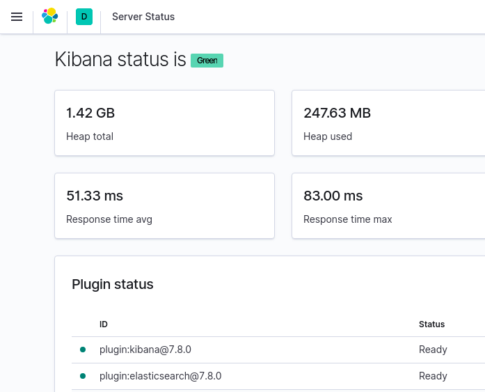
Now navigate in the browser to the URL: https://192.168.99.102:31112/status to check that the web UI is running and Elasticsearch is connected properly.

Note: The IP address 192.168.99.102 is the value returned when running the command minikube ip on its own.

Deploying Logstash

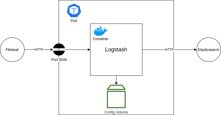
The next step is to get Logstash running within our setup. Logstash will operate as the tool that will collect logs from our application and send them through to Elasticsearch. It provides various benefits for filtering and re-formatting log messages, as well as collecting from various sources and outputting to various destinations. For this tutorial, we are only interested in using it as a pass-through log collector and forwarder.

In the above diagram, you can see our desired setup. We are aiming to deploy a Logstash container into a new Pod. This container will be configured to listen on port 5044 for log entries being sent from a Filebeat application (more on this later). Those log messages will then be forwarded straight onto our Elasticsearch Kibana Logstash instance that we setup earlier, via the HTTP port that we have exposed.

To achieve this setup, we are going to have to leverage the Kubernetes YAML files. This is a more verbose way of creating deployments and can be used to describe various resources (such as Deployments, Services, etc) and create them through a single command. The reason we need to use this here is that we need to configure a volume for our Logstash container to access, which is not possible through the CLI commands. Similarly, we could have also used this approach to reduce the number of steps required for the earlier setup of Elasticsearch and Kibana; namely the configuration of environment variables and separate steps to create Service resources to expose the ports into the containers.

So, let’s begin – create a file called logstash.conf and enter the following:

input {
  beats {
    port => "5044"
  }
}
 
output {
  elasticsearch {
    hosts => ["https://192.168.99.102:30445"]
    index => "%{[@metadata][beat]}-%{[@metadata][version]}-%{+YYYY.MM.dd}"
  }
  stdout {
    codec => rubydebug
  }
}

Note: The IP and port combination used for the Elasticsearch hosts parameter come from the Minikube IP and exposed NodePort number of the Elasticsearch Service resource in Kubernetes.

Next, we need to create a new file called deployment.yml. Enter the following Kubernetes Deployment resource YAML contents to describe our Logstash Deployment.

---
kind: Deployment
apiVersion: apps/v1
metadata:
  name: log-manual
spec:
  replicas: 1
  selector:
    matchLabels:
      name: log-manual
  template:
    metadata:
      labels:
        name: log-manual
    spec:
      hostname: log-manual
  containers:
   - name: log-manual
     ports:
     - containerPort: 5044
       name: filebeat
       image: logstash:7.8.0
     volumeMounts:
     - name: log-manual-pipeline
       mountPath: /usr/share/logstash/pipeline/
     command:
     - logstash
     volumes:
      - name: log-manual-pipeline
     configMap:
       name: log-manual-pipeline
       items:
       - key: logstash.conf
         path: logstash.conf
---

You may notice that this Deployment file references a ConfigMap volume. Before we create the Deployment resource from this file, we need to create this ConfigMap. This volume will contain the logstash.conf file we have created, which will be mapped to the pipeline configuration folder within the Logstash container. This will be used to configure our required pass-through pipeline. So, run the following command:

$ kubectl create configmap log-manual-pipeline 
--from-file ./logstash.conf

[Output]
configmap/log-manual-pipeline created

We can now create the Deployment resource from our deployment.yml file.

$ kubectl create –f ./deployment.yml

[Output]
deployment.apps/log-manual created

To check that our Logstash instance is running properly, follow the logs from the newly created Pod.

$ kubectl get pods

[Output]
NAME                          READY   STATUS    RESTARTS   AGE
es-manual-7d8bc4cf88-b2qr9    1/1     Running   3          7d2h
kib-manual-7c7f848654-z5f9c   1/1     Running   1          3d23h
log-manual-5c95bd7497-ldblg   1/1     Running   0          4s

$ kubectl logs –f log-manual-5c95bd7497-ldblg

[Output]
...
... Beats inputs: Starting input listener {:address=>"0.0.0.0:5044"}
... Pipeline started {"pipeline.id"=>"main"}
... Pipelines running {:count=>1, :running_pipelines=>[:main], :non_running_pipelines=>[]}
... Starting server on port: 5044
... Successfully started Logstash API endpoint {:port=>9600}

Note: You may notice errors stating there are “No Available Connections” to the Elasticsearch instance endpoint with the URL https://elasticsearch:9200/. This comes from some default configuration within the Docker Image, but does not affect our pipeline, so can be ignored in this case.

Expose the Logstash Filebeats port

Now that Logstash is running and listening on container port 5044 for Filebeats log message entries, we need to make sure this port is mapped through to the host so that we can configure a Filebeats instance in the next section. To achieve this, we need another Service resource to expose the port on the Minikube host. We could have done this inside the same deployment.yml file, but it’s worth using the same approach as before to show how the resource descriptor and CLI commands can be used in conjunction.

As with the earlier steps, run the following command to expose the Logstash Deployment through a Service resource.

$ kubectl expose deployment log-manual 
--type NodePort --port 5044

[Output]
service/log-manual exposed

Now check that the Service has been created and the port has been mapped properly.

$ kubectl get services

[Output]
NAME         TYPE        CLUSTER-IP      EXTERNAL-IP   PORT(S)
es-manual    NodePort    10.96.114.186           9200:30445/TCP
kib-manual   NodePort    10.96.112.148           5601:31112/TCP
kubernetes   ClusterIP   10.96.0.1               443/TCP
log-manual   NodePort    10.96.254.84            5044:31010/TCP

As you can see, the container port 5044 has been mapped to port 31010 on the host. Now we can move onto the final step: configuring our application and a Sidecar Filebeats container to pump out log messages to be routed through our Logstash instance into Elasticsearch.

Application

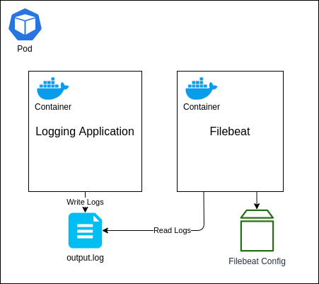
Right, it’s time to setup the final component: our application. As I mentioned in the previous section, we will be using another Elastic Stack component called Filebeats, which will be used to monitor the log entries written by our application into a log file and then forward them onto Logstash.

There are a number of different ways we could structure this, but the approach I am going to walk through is by deploying both our application and the Filebeat instance as separate containers within the same Pod. We will then use a Kubernetes volume known as an Empty Directory to share access to the log file that the application will write to and Filebeats will read from. The reason for using this type of volume is that its lifecycle will be directly linked to the Pod. If you wish to persist the log data outside of the Pod, so that if the Pod is terminated and re-created the volume remains, then I would suggest looking at another volume type, such as the Local volume.

To begin with, we are going to create the configuration file for the Filebeats instance to use. Create a file named filebeat.yml and enter the following contents.

filebeat.inputs:
 - type: log
   paths:
    - /tmp/output.log
 
output:
  logstash:
    hosts: [ "192.168.99.102:31010" ]

This will tell Filebeat to monitor the file /tmp/output.log (which will be located within the shared volume) and then output all log messages to our Logstash instance (notice how we have used the IP address and port number for Minikube here).

Now we need to create a ConfigMap volume from this file.

$ kubectl create configmap beat-manual-config 
--from-file ./filebeat.yml

[Output]
configmap/beat-manual-config created

Next, we need to create our Pod with the double container setup. For this, similar to the last section, we are going to create a deployment.yml file. This file will describe our complete setup so we can build both containers together using a single command. Create the file with the following contents:

kind: Deployment
  apiVersion: apps/v1
  metadata:
    name: logging-app-manual
  spec:
    replicas: 1
    selector:
      matchLabels:
        name: logging-app-manual
  template:
    metadata:
      labels:
        name: logging-app-manual
    spec:
      hostname: logging-app-manual
      containers:
        - name: beat-manual
          image: elastic/filebeat:7.8.0
          args: [
            "-c", "/etc/filebeat/filebeat.yml",
            "-e"
          ]
          volumeMounts:
            - name: beat-manual-config
              mountPath: /etc/filebeat/
            - name: manual-log-directory
              mountPath: /tmp/
        - name: logging-app-manual
          image: sladesoftware/log-application:latest
          volumeMounts:
            - name: manual-log-directory
              mountPath: /tmp/
      volumes:
        - name: beat-manual-config
          configMap:
            name: beat-manual-config
            items:
              - key: filebeat.yml
                path: filebeat.yml
        - name: manual-log-directory
          emptyDir: {}

I won’t go into too much detail here about how this works, but to give a brief overview this will create both of our containers within a single Pod. Both containers will share a folder mapped to the /tmp path, which is where the log file will be written to and read from. The Filebeat container will also use the ConfigMap volume that we have just created, which we have specified for the Filebeat instance to read the configuration file from; overwriting the default configuration.

You will also notice that our application container is using the Docker Image <code>sladesoftware/log-application:latest. This is a simple Docker Image I have created that builds on an Alpine Linux image and runs an infinite loop command that appends a small JSON object to the output file every few seconds.

To create this Deployment resource, run the following command:

$ kubectl create –f ./deployment.yml

[Output]
deployment.apps/logging-app-manual created

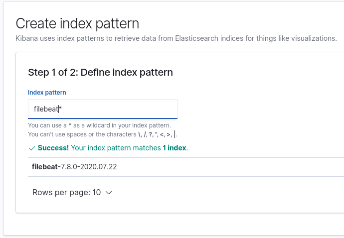
And that’s it! You should now be able to browse to the Kibana dashboard in your web browser to view the logs coming in. Make sure you first create an Index Pattern to read these logs – you should need a format like filebeat*.

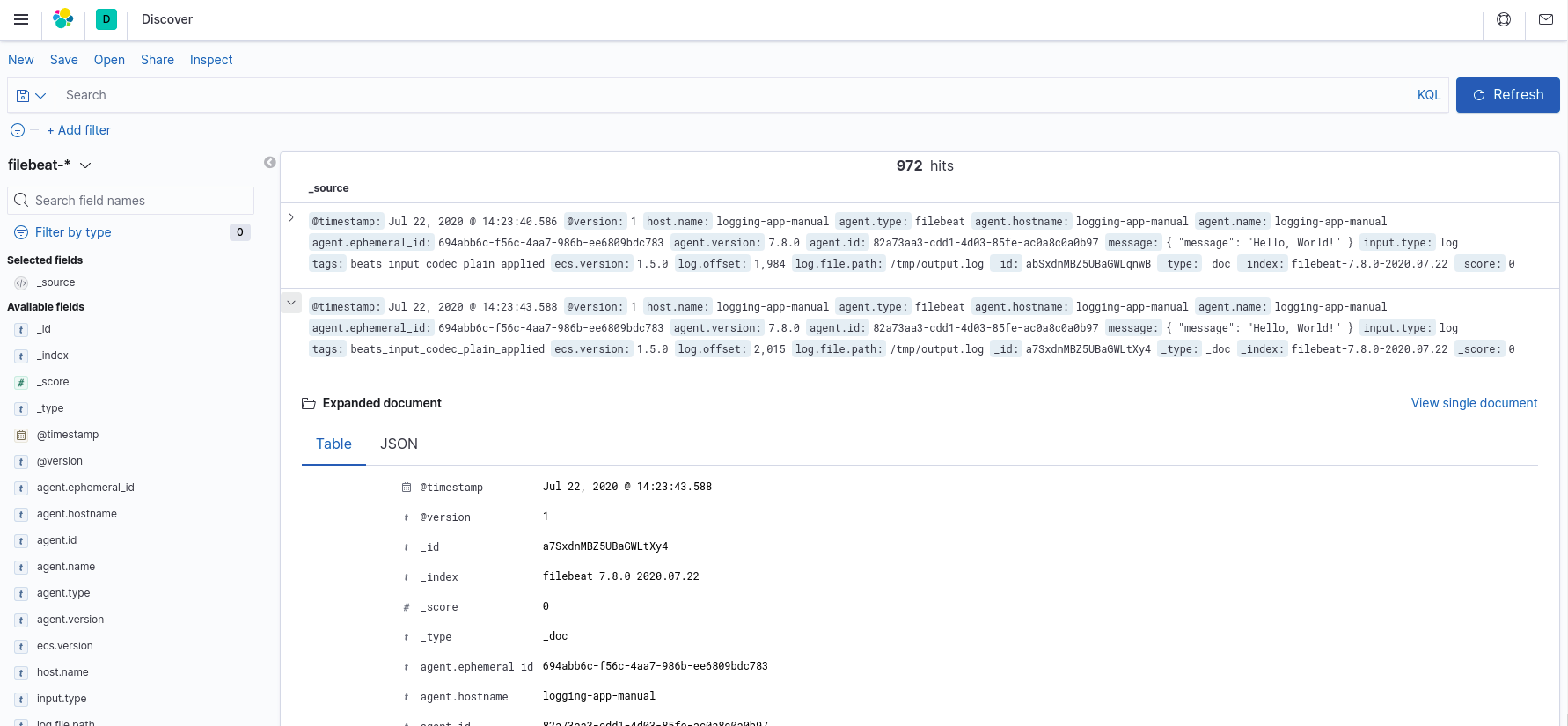
Once you have created this Index Pattern, you should be able to view the log messages as they come into Elasticsearch over on the Discover page of Kibana.

Using Helm charts

If you have gone through the manual tutorial, you should now have a working Elastic Stack setup with an application outputting log messages that are collected and stored in Elasticsearch and viewable in Kibana. However, all of that was done through a series of commands using the Kubernetes CLI, and Kubernetes resource description files written in YAML. Which is all a bit tedious.

The aim of this section is to achieve the exact same Elastic Stack setup as before, only this time we will be using something called Helm. This is a technology built for making it easier to setup applications within a Kubernetes cluster. Using this approach, we will configure our setup configuration as a package known as a Helm Chart, and deploy our entire setup into Kubernetes with a single command!

I won’t go into a lot of detail here, as most of what will be included has already been discussed in the previous section. One point to mention is that Helm Charts are comprised of Templates. These templates are the same YAML files used to describe Kubernetes resources, with one exception: they can include the Helm template syntax, which allows us to pass through values from another file, and apply special conditions. We will only be using the syntax for value substitution here, but if you want more information about how this works, you can find more in the official documentation.

Let’s begin. Helm Charts take a specific folder structure. You can either use the Helm CLI to create a new Chart for you (by running the command helm create <NAME>), or you can set this up manually. Since the creation command also creates a load of example files that we aren’t going to need, we will go with the manual approach for now. As such, simply create the following file structure:

.
├── Chart.yaml
├── filebeat.yml
├── logstash.conf
├── templates
│   ├── elasticsearch.yaml
│   ├── kibana.yaml
│   ├── logging-app-and-filebeat.yaml
│   └── logstash.yaml
└── values.yaml

Now, follow through each of the following files, entering in the contents given. You should see that the YAML files under the templates/ folder are very familiar, except that they now contain the Service and ConfigMap definitions that we previously created using the Kubernetes CLI.

Chart.yaml

apiVersion: v2
name: elk-auto
description: A Helm chart for Kubernetes
type: application
version: 0.1.0

This file defines the metadata for the Chart. You can see that it indicates which version of the Kubernetes API it is using. It also names and describes the application. This is similar to a package.json file in a Node.js project in that it defines metadata used when packaging the Chart into a redistributable and publishable format. When installing Charts from a repository, it is this metadata that is used to find and describe said Charts. For now, though, what we enter here isn’t very important as we won’t be packaging or publishing the Chart.

filebeat.yml

filebeat.inputs:
  - type: log
    paths:
      - /tmp/output.log
 
output:
  logstash:
    hosts: [ "${LOGSTASH_HOSTS}" ]

This is the same Filebeat configuration file we used in the previous section. The only difference is that we have replaced the previously hard-coded Logstash URL with the environment variable: LOGSTASH_HOSTS. This will be set within the Filebeat template and resolved during Chart installation.

logstash.conf

input {
  beats {
    port => "5044"
  }
}
 
output {
  elasticsearch {
    hosts => ["${ELASTICSEARCH_HOSTS}"]
    index => "%{[@metadata][beat]}-%{[@metadata][version]}-%{+YYYY.MM.dd}"
  }
  stdout {
    codec => rubydebug
  }
}

This is the same Logstash configuration file we used previously. The only modification, is that we have replaced the previously hard-coded Elasticsearch URL with the environment variable: ELASTICSEARCH_HOSTS. This variable is set within the template file and will be resolved during Chart installation.

templates/elasticsearch.yaml

apiVersion: apps/v1
kind: Deployment
metadata:
  name: es-auto
  labels:
    name: es-auto
spec:
  replicas: 1
  selector:
    matchLabels:
      name: es-auto
  template:
    metadata:
      labels:
        name: es-auto
    spec:
      containers:
        - name: es-auto
           image: elasticsearch:7.8.0
           ports:
            - containerPort: 9200
               name: http
           env:
            - name: discovery.type
               value: single-node
  ---
apiVersion: v1
kind: Service
metadata:
  labels:
    name: es-auto
  name: es-auto
spec:
  selector:
    name: es-auto
  type: NodePort
  ports:
    - nodePort: {{ .Values.ports.elasticsearch }}
      port: 9200
      protocol: TCP
      targetPort: 9200

Here, we are creating 2 Kubernetes resources:

  • A Deployment that spins up 1 Pod containing the Elasticsearch container
  • A Service that exposes the Elasticsearch port 9200 on the host (Minikube) that both Logstash and Kibana will use to communicate with Elasticsearch via HTTP

templates/kibana.yaml

apiVersion: apps/v1
kind: Deployment
metadata:
  name: kib-auto
  labels:
    name: kib-auto
spec:
  replicas: 1
  selector:
    matchLabels:
      name: kib-auto
  template:
    metadata:
      labels:
         name: kib-auto
    spec:
      containers:
        - name: kib-auto
           image: kibana:7.8.0
           ports:
             - containerPort: 5601
               name: http
           env:
            - name: ELASTICSEARCH_HOSTS
               value: https://{{ .Values.global.hostIp }}:{{ .Values.ports.elasticsearch }}
---
apiVersion: v1
kind: Service
metadata:
  name: kib-auto
  labels:
    name: kib-auto
spec:
  selector:
    name: kib-auto
  type: NodePort
  ports:
    - nodePort: {{ .Values.ports.kibana }}
      port: 5601
      protocol: TCP
      targetPort: 5601

Here, we are creating 2 Kubernetes resources:

  • A Deployment that spins up 1 Pod containing the Kibana container; configured to point to our exposed Elasticsearch instance
  • A Service that exposes the Kibana port 5601 on the host (Minikube) so that we can view the Kibana Dashboard via the web browser

templates/logging-app-and-filebeat.yaml

apiVersion: apps/v1
kind: Deployment
metadata:
  name: app-auto
  labels:
    name: app-auto
spec:
  replicas: 1
  selector:
    matchLabels:
      name: app-auto
  template:
    metadata:
      labels:
        name: app-auto
    spec:
      containers:
      - name: app-auto
         image: sladesoftware/log-application:latest
         volumeMounts:
         - name: log-output
           mountPath: /tmp/
      - name: beat-auto
         image: elastic/filebeat:7.8.0
         env:
         - name: LOGSTASH_HOSTS
           value: {{ .Values.global.hostIp }}:{{ .Values.ports.logstash }}
         args: [
           "-c", "/etc/filebeat/filebeat.yml",
           "-e"
         ]
         volumeMounts:
         - name: log-output
           mountPath: /tmp/
         - name: beat-config
           mountPath: /etc/filebeat/
      volumes:
      - name: log-output
         emptyDir: {}
      - name: beat-config
         configMap:
           name: beat-config
           items:
           - key: filebeat.yml
             path: filebeat.yml
---
apiVersion: v1
kind: ConfigMap
metadata:
  name: beat-config
data:
  filebeat.yml: |
{{ .Files.Get "filebeat.yml" | indent 4 }}

Here, we are creating 2 Kubernetes resources:

  • A Deployment, which spins up 1 Pod containing 2 containers: 1 for our application and another for Filebeat; the latter of which is configured to point to our exposed Logstash instance
  • A ConfigMap containing the Filebeat configuration file

We can also see that a Pod-level empty directory volume has been configured to allow both containers to access the same /tmp directory. This is where the output.log file will be written to from our application, and read from by Filebeat.

templates/logstash.yaml

apiVersion: apps/v1
kind: Deployment
metadata:
  name: log-auto
  labels:
    name: log-auto
spec:
  replicas: 1
  selector:
    matchLabels:
      name: log-auto
  template:
    metadata:
      labels:
        name: log-auto
    spec:
      containers:
        - name: log-auto
           image: logstash:7.8.0
           ports:
             - containerPort: 5044
               name: filebeat
           env:
             - name: ELASTICSEARCH_HOSTS
               value: https://{{ .Values.global.hostIp }}:{{ .Values.ports.elasticsearch }}
           volumeMounts:
             - name: log-auto-pipeline
               mountPath: /usr/share/logstash/pipeline/
           command:
             - logstash
      volumes:
        - name: log-auto-pipeline
           configMap:
            name: log-auto-pipeline
            items:
              - key: logstash.conf
                path: logstash.conf
---
apiVersion: v1
kind: ConfigMap
metadata:
  name: log-auto-pipeline
data:
  logstash.conf: |
{{ .Files.Get "logstash.conf" | indent 4 }}
---
apiVersion: v1
kind: Service
metadata:
  name: log-auto
  labels:
    name: log-auto
spec:
  selector:
    name: log-auto
  type: NodePort
  ports:
  - nodePort: {{ .Values.ports.logstash }}
    port: 5044
    protocol: TCP
    targetPort: 5044

Here, we can see that we have created 3 Kubernetes resources:

  • A Deployment, which spins up 1 Pod containing the Logstash container; configured to point to our exposed Elasticsearch instance
  • A ConfigMap containing the Logstash configuration file
  • A Service to expose the Logstash port 5044 on the host so that Filebeat can access it via HTTP

values.yaml

global:
  hostIp: 127.0.0.1
 
ports:
  elasticsearch: 31996
  kibana: 31997
  logstash: 31998

This file contains the default values for all of the variables that are accessed in each of the template files. You can see that we have explicitly defined the ports we wish to map the container ports to on the host (I.e. Minikube). The hostIp variable allows us to inject the Minikube IP when we install the Chart. You may take a different approach in production, but this satisfies the aim of this tutorial.

Now that you have created each of those files in the aforementioned folder structure, run the following Helm command to install this Chart into your Kubernetes cluster.

$ helm install elk-auto . --set global.hostIp=$(minikube ip)

[Output]
NAME: elk-auto
LAST DEPLOYED: Fri Jul 24 12:40:21 2020
NAMESPACE: default
STATUS: deployed
REVISION: 1
TEST SUITE: None

Give it a few minutes for all of the components fully start up (you can check the container logs through the Kubernetes CLI if you want to watch it start up) and then navigate to the URL https://<MINIKUBE IP>:31997 to view the Kibana dashboard. Go through the same steps as before with creating an Index Pattern and you should now see your logs coming through the same as before.

That’s it! We have managed to setup the Elastic Stack within a Kubernetes cluster. We achieved this in two ways: manually by running individual Kubernetes CLI commands and writing some resource descriptor files, and sort of automatically by creating a Helm Chart; describing each resource and then installing the Chart using a single command to setup the entire infrastructure. One of the biggest benefits of using a Helm Chart approach is that all resources are properly configured (such as with environment variables) from the start, rather than the manual approach we took where we had to spin up Pods and containers first in an erroring state, then reconfigure the environment variables, and wait for them to be terminated and re-spun up.

What’s next?

Now we have seen how to set up the Elastic Stack within a Kubernetes cluster, where do we go with it next? The Elastic Stack is a great tool to use when setting up a centralized logging approach. You can delve more into this by reading this article that describes how to use a similar setup but covers a few different logging techniques. Beyond this, there is a wealth of information out there to help take this setup to production environments and also explore further options regarding packaging and publishing Helm Charts and building your resources as a set of reusable Charts.

Overcoming DNS barriers for Kubernetes Scaling

It was a cloudy winter morning when I had arrived at the office and found, to our horror, that a Kubernetes cluster was suffering from extremely high CPU and network usage and had become almost completely non-functional.

To make things worse, restarting the nodes (the go-to DevOp solution), seemed to have absolutely no effect on the issue. Something was poisoning the network and we had to find out what it was and fast.

The first thing we did was look at the logs and sure enough, we discovered an out of memory message:

Now, before resorting to any dark and perhaps satanic rituals that involve sacrificing children, we decided to run “top” (the Linux tool) on one of the nodes to understand it better.

The result really knocked us off our feet: a process named “protokube” which usually behaves nicely all of a sudden went berserk and started consuming between 200% to 300% of CPU usage. We also ran “netstat -plan | grep <protokube_pid>” to see which ports it was listening to or communicating on and found out it was port 3999/TCP.

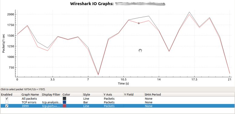
That was suspicious indeed but we wanted to be certain that we found the real culprit, so we ran tcpdump to capture some traffic from one of the nodes on port 3999/TCP and then used Wireshark to understand how much of the total traffic was generated by Protokube.

From the chart above it’s evident that most of the node’s traffic actually goes through port 3999, which means that it’s being sent and received by the Protokube process. So, we knew that this process was responsible for the issue, but what does the process do in the first place?

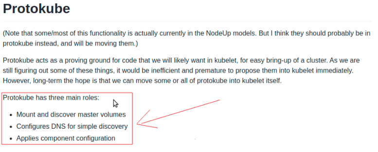
A quick google search and we could clearly see the list of Protokube’s tasks:

It soon became clear that we could rule out the first and last tasks as they’re most likely not related to our case. This left us with “Configures DNS for simple discovery” but how does it actually work?

Our next step was to find out what useful information we could get from the traffic data to better understand how Protokube configures DNS for simple discovery.

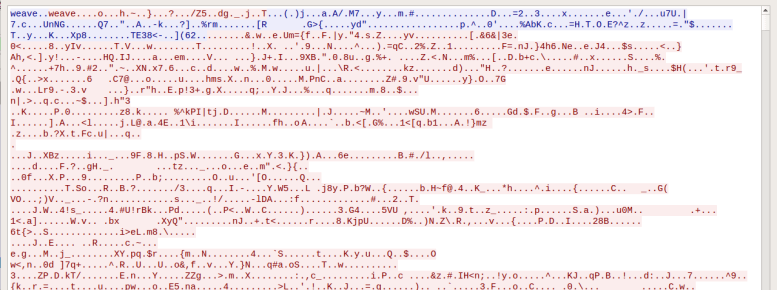
While reviewing the raw traffic in Wireshark and looking for clues, we noticed the following communication:

As you can see above, the communication starts with the text “weave..weave”. After searching we found that this type of Protokube traffic uses the Weave library internally.

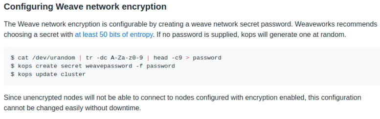
So now we understand why we couldn’t decipher the raw traffic (i.e. due to the Weave network encryption), but we’re still left with the original question of how Protokube configures the DNS for simple discovery?

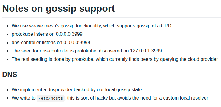
A few more searches and a few cups of tea later we found that Protokube uses Gossip DNS encrypted with Weave and runs on port 3999/TCP and 3998/TCP. For those who aren’t familiar, Gossip is designed to handle name resolution in a decentralized manner to keep up with fast-changing containerized environments.

Now that we finally knew what the Protokube process actually did and how it related to the traffic we saw on port 3999/TCP, there was still the original question we needed to answer: why was the Protokube process behaving so badly and how to address it?

To find the answer, we had to look deeper and analyze the actual communication between the nodes on port 3999/TCP. Here’s an example of communication we found:

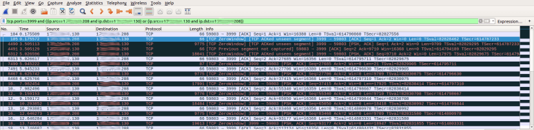
As you can see from the above screenshot, the communication starts with the node 1xx.xx.xx.130 that tries to connect to the node at 1xx.xx.xx.208 on port 3999/TCP at packet no. 6313 and as soon as it’s ready to send Gossip DNS  data, the node at 1xx.xx.xx.208 responds with a zero-length TCP Window Size.

What exactly is a TCP window size? The TCP window size is a throttling mechanism built into the TCP protocol to avoid overloading the recipient. In order to demonstrate this, let’s consider the following example. Computer A wants to send data to computer B over TCP port 3999. Here’s how the communication will typically look like:

  1. Computer A: SYN source port = X, destination port = 3999 (connection request)
  2. Computer B: SYN-ACK source port = 3999, destination port X (acknowledgment of connection request)
  3. Computer A: ACK source port = X, destination port = 3999 (acknowledgment of the request, which essentially opens the connection)
  4. Computer A: PSH destination port = 3999, destination port X (data pushed to recipient)

But what happens if, for example, computer B cannot handle the incoming traffic at that particular moment (e.g. due to temporary server overload)?

This is exactly what the TCP Window Size aims to solve. In every packet that is sent by the client or server,  it specifies a Window Size that is set by the packet sender to indicate how many bytes the sender is willing to accept in return.

When the TCP window size reaches zero (due to overload or hacking), the recipient of the packet will periodically poll the sender of the packet to see if it has become available again (i.e. if the Window Size has since grown) and if it has, the sender will finally send the requested data.

It’s absolutely normal for computers to become busy at times and use this mechanism to throttle their communications.

However, in our case, since the Protokube Gossip DNS uses a mesh topology, things can look very different and that’s exactly what happened in our case:

  1. Computer A=>B: SYN (source port = X, destination port = 3999)
  2. Computer B=>A: SYN-ACK (source port = 3999, destination port X)
  3. Computer A=>B: ACK (source port = X, destination port = 3999)
  4. Computer A=>B: PSH (source port = X, destination port = 3999) With the data that needs to be transmitted
  5. Computer B=>A: PSH-ACK (source port = 3999, destination port X)It will respond with a TCP Window Size of 0 because of some unrelated temporary heavy load. Now, Computer A cannot send the data, causing it to periodically poll Computer B.
    .
    .
    .
  6. Computer C=>B: SYN (source port = Y, destination port = 3999)
  7. Computer B=>C: SYN-ACK (source port = 3999, destination port Y)
  8. Computer C=>B: ACK (source port = Y, destination port = 3999)
  9. Computer C=>B: PSH (source port = Y, destination port = 3999) With the data that needs to be transmitted
  10. Computer B=>C: PSH-ACK (source port = 3999, destination port Y) with the TCP Window Size set to 0 because of some unrelated temporary heavy load

In our mesh topology, if computer B becomes temporarily busy for any reason, it will immediately overload all connections in its DNS Gossip network because all nodes that try to publish their DNS cache to computer B will become overloaded by other nodes trying to poll it at the same time. This resulted in a cascade of overloads that was made worse as more nodes got added to the network. More nodes meant exponentially more connections.

Due to the constant polling as a consequence of even a small initial overload, a small issue eventually spiraled to a point where the window size reached 0 and the network would come to a halt.  

The solution I discovered was to run a script that loops through all nodes in a cluster, connects to them and kills the Protokube Daemon to force Kubernetes to restart every Protokub pod. The script ran pretty fast allowing for more nodes to become available and respond to the Gossip requests. After all nodes on the cluster went through this process, the cluster was back online and the extremely heavy load diminished.

We also reduced the number of servers by using more powerful ones. This reduced the overall node count and possible connections on the Gossip mesh thereby lowering the risk of overloading it.

Fewer nodes means less gossip which means less chance of failure.

Although this indeed solved the problem, the real long-term solution for production environments is to abandon Gossip DNS completely and switch to better techniques such as the AWS Route53 service.

Just as a side note, the very same throttling mechanism can and is being used by hackers to attack servers and services by causing a DoS attack. The idea is by sending multiple request packets to a server and setting the TCP window size to zero or to a low value, it forces the server to hold the connection open for long periods of time. Such attacks are known as Socketstress. A similar attack that operates in higher layers of the communication is the Slowloris attack. This works by requesting a resource but doesn’t allow the server to return it properly – causing a large number of connections to be left open and idle.

To summarize, we initially thought we needed to increase nodes to handle our growing needs, but this caused the network to come to a halt. After investigating, we found the culprit to be the way Gossip DNS is implemented in Protokube. Counter-intuitively, by reducing the number of nodes and forcing K8s to restart all Protokube pods in a cluster, we were able to scale without sacrificing performance (or any children). However, even this was a short-term solution and we eventually abandoned Gossip DNS for a dedicated DNS server.

EKS vs. KOPS

In the past, applications would be deployed by installation on a host, using the operating system package manager. This was a heavy solution with tremendous reliance on the operating system package manager and increased complexity with libraries, configuration, executables and so on all interconnected.

Then came containers. Containers are small and fast, and are isolated from each other and from the host. Containers have numerous benefits, such as continuous development and deployment, agile application creation,  and increased portability to name just a few.

Enter Kubernetes, or “K8”. Kubernetes is “a portable, extensible open-source platform for managing containerized workloads and services, that facilitates both declarative configuration and automation” and is used extensively, including by IBM, eBay and SAP.

Kubernetes, Containers and AWS

A containerized application typically consists of many containers. There might be a container for the application itself, for a database, and so on. This environment could be built and tested on a single host, however this can quickly become problematic if there is an issue when in production.

Thus a multi-container application can be deployed on multiple hosts. But how does one manage these? A specialized tool is required, which is where “container orchestration” comes in. When it comes to container orchestration and Amazon Web Services (AWS), one of the most popular is the aforementioned Kubernetes. There are many ways to run a Kubernetes cluster on AWS, and we’ll look at two major ones: kops, and EKS.

Kops

Kubernetes Operations, or “kops” is a set of tools for installing, operating, and deleting Kubernetes clusters in the cloud. It is billed as “the easiest way to get a production grade Kubernetes cluster up and running”. Users include PlayCom and Spreaker.

What’s great about kops is that it gives powerful functionality (you can create, delete, and maintain Kubernetes clusters) from the command line.

It officially supports AWS of course, which is another benefit.

With kops, you can have fully automated installation, support for custom Kubernetes add-ons, autocompletion in the command line, self-healing functionality, and support for most operating systems.

EKS

Amazon Elastic Container Service for Kubernetes, known as EKS, allows the deployment, management, and scaling of containerized applications, using Kubernetes, on AWS.

EKS runs the Kubernetes management infrastructure across multiple AWS availability zones, eliminating that single point of failure referenced previously. Companies using EKS include GoDaddy, Skyscanner, Verizon, Snapchat, and many other giants.

EKS can be used for running microservices applications, hybrid container deployments, batch processing and application migration (you can containerize and migrate existing applications to EKS without needing to refactor code or tooling).

What are some of the benefits of Amazon EKS? For one, EKS is certified Kubernetes conformant, so applications managed by EKS are fully compatible with applications managed by any standard Kubernetes environment. Another benefit is that EKS provides on-demand upgrades and patching, and there is no control plane to manage.

Different Horses For Different Courses

Which to choose? Both of these options are powerful, market-tested and have great integration with AWS.

Amazon EKS launched at AWS re:Invent in December of 2017. Amazon rigorously tested it for 6 months before general release, so as to ensure reliability, and that is would be a realistic alternative to kops which is generally well-liked by the Kubernetes community and is open source. This is perhaps one of the reasons that take-up of EKS is taking longer than some people expected.

There is good reason for this however. As The New Stack reports, “One of the reasons why EKS is taking a longer time to become generally available is the integration with existing building blocks of AWS. From VPC networking to IAM, Amazon has carefully integrated the core services without breaking the expected behavior. Customers can also take advantage of standard monitoring and logging tools such as CloudWatch and CloudTrail for logging and monitoring EKS workloads. Amazon EKS passed the Cloud Native Computing Foundation conformance test to become a certified hosted platform, which means that all the plugins and extensions that work with upstream Kubernetes will work as is in EKS.”

Certainly kops is very easy to use, there is a tremendous amount of community support and literature around to assist users, and it is well designed for creating, deleting, customizing, upgrading and maintaining Kubernetes clusters.

Kops has the typical advantages and drawbacks of battle-hardened open source solutions, and certainly gets the job done. With EKS, the “new kid on the block”, Amazon has built a powerful tool that packs a powerful punch when it comes to functionality and integrations, including with popular AWS services such as their IAM.

In the end, if your organization is already deeply integrated with AWS, EKS could be a great option going forward. Like other Amazon services, keep an eye on costs, as scaling happens quickly and costs can escalate sharply. But don’t disregard kops just yet: it has proven itself as a solid performer that gets the job done.

Anyway you choose, be sure to check out Coralogix’s predefined image for K8 log collection, it includes all your K8 metadata and helps you get started in no time.

Terraform vs Helm Charts

Since Docker first came onto the scene in 2013 and really popularized containerization, many organizations have chosen to deploy cloud workloads using Docker containers.

Containers come with numerous benefits over running applications directly inside of a virtual machine hypervisor, including significantly portability benefits and efficiencies in terms of storage and overhead.

Docker provides a runtime for running containerized applications, in addition to a format for encapsulating and delivering applications in containers.

With the increasing adoption of containerization, the need arose to manage, schedule and control clusters of containers, and that’s where Kubernetes comes in. Kubernetes is an open-source system for automating deployment, scaling, and management of containerized applications, generally being Docker containers.

When interfacing with Kubernetes, 2 competing tools are often discussed: Terraform, and Helm.

Terraform

Terraform is a tool for building, changing, and versioning infrastructure safely and efficiently. Terraform can manage existing providers, as well as custom in-house solutions.

Terraform

For example, in large-scale infrastructures, static assignment of applications to machines becomes a challenge. To solve this, there are a number of schedulers like the aforementioned Kubernetes that can be used to dynamically schedule Docker containers. Resource schedulers can be treated as a provider, which allows Terraform to request resources from them, enabling Terraform to be used in layers; setting up the physical infrastructure running the schedulers, and provisioning onto the scheduled grid.

Configuration management is critical in the software development ecosystem, and while people have used platforms like Chef or Puppet for this purpose, Terraform adds a whole new dimension.

Key features of Terraform include:

Infrastructure as Code: Infrastructure as code (or IaC) is the process of managing and provisioning computer data centers through machine-readable definition files, rather than physical hardware configuration or interactive configuration tools. With Terraform, infrastructure is described using a high-level configuration syntax, allowing a blueprint of your data center to be versioned and treated as you would any other code.

Smoothness through cloud provider’s API

Terraform actually uses the cloud provider’s API, which makes the whole process a lot smoother, and more effective in terms of maintainability, ease and security.

Stability and efficiency through immutable infrastructure

Forget about configuration drift and bugs. Terraform uses the immutable infrastructure approach, where servers are replaced rather than changed. This means simplified operations, fewer failures, and fewer errors, threats, and vulnerabilities.

Simplicity through code

With server provisioning, Terraform leaves issues pertaining to software container deployment to Docker. The cloud infrastructure is seen as code, bringing additional advantages.

Effectiveness through declarative code style

With a declarative code style (imperative programming: how you do something, declarative programming: what you do/what the end state should be), meaning advantages when it comes to succinctness, speed, and fewer complications.

Terraform works with any cloud-based setup, so it doesn’t matter if it’s public cloud or an on-premise-based setup.

It allows:

Execution Plans: Use the planning step to see what will happen when you call apply, avoiding nasty surprises.

Resource Graph: Builds a graph of all your resources, and build infrastructure as efficiently as possible.

Change Automation: Apply changesets to your infrastructure automatically, conserving resources and avoiding errors.

Terraform is open source, with strong community engagement.

Helm

Helm helps users manage Kubernetes applications, and Helm Charts assists users in defining, installing, and upgrading Kubernetes applications.

helm

Helm is maintained by the CNCF in collaboration with Microsoft, Google, Bitnami and the Helm contributor community.

Keeping with the nautical theme of docking, containers and quays, Helm enables Kubernetes users greater control over their cluster, just like the captain of a ship at the helm.

Helm Charts provide the ability to leverage Kubernetes packages when building and deploying applications through a click or single CLI command. When a user executes the Helm install command, a Tiller (yes, another maritime reference) Server receives the incoming request, installing the appropriate package into the Kubernetes cluster. These packages are called Charts.

A chart can have deployments, configmaps, services, and so on defined as yaml files, which are templates. You can define certain charts as dependencies for other charts, or nest charts inside others.

Helm has a number of advantages:

  • Deploy and manage manifests in a production environment
  • Complex applications can be packaged together
  • Rollback or upgrade multiple objects together
  • An extensive and reusable pre-built chart repository
  • Easily change parameters of templates
  • Deploy to multiple environments easily

Helm has been praised by users for its vibrant community, its ability to manage complex apps, in-place upgrades and custom hooks for hassle-free updates, the ability to share Chart, and easy rollbacks.

Terraform vs Helm

Both Terraform and Helmchart have a number of similarities, as well as some differences.

In terms of similarities, they allow you to describe and maintain Kubernetes objects as code, they support modularity, have a curated list of packages, allow you to see the impact of changes before running them, and allow installation from sources like git repositories or local directories.

In terms of differences, Terraform does not install anything within the Kubernetes cluster itself, while Helm installs Tiller within the cluster. Helm cannot install a Kubernetes cluster, while Terraform can. When it comes to modularity Terraform uses modules while Helm uses sub-charts, and Terraform uses the JSON/HCL file format while Helm uses standard manifests and Go-templates.

Both Terraform and Helm have their advantages and disadvantages. For example, because Terraform uses the same tool and codebase for both infrastructure and cluster management, there is not too much of a learning curve when it comes to using it with Kubernetes. Terraform is also relatively new with its Kubernetes interfacing, so there are some kinks and issues. On the other hand, rolling back with Helm is a lot easier, but maintaining it can take up precious resources.

The safe option is to go with Helm, as it has been around for a while and has proven itself, not to mention the support of some serious players behind its continuing development. Terraform is improving rapidly, however, and can do a lot of the heavy lifting for you.

Using the Tools to Add Value

The debate is likely to rage on for a while, but what cannot be disputed is the popularity of Kubernetes, and the value it can add to any organization. The great news is that with some simple integrations, there are configuration management tools available that can take Kubernetes to a whole new level. Coralogix can be integrated into Kubernetes logs with a pre-set image so that you can take advantage of everything the platform has to offer: including mapping software flows, automatically detecting production problems, delivering pinpoint insights and providing top-level visibility.