The new standard of observability is here. Discover Olly, the industry’s first

Elasticsearch is a popular distributed search and analytics engine designed to handle large volumes of data for fast, real-time searches. Elasticsearch’s capabilities make it useful in many essential cases like log analysis. Its users can create their own analytics queries, or use existing platforms like Coralogix to streamline analyzing data stored in an index.
We’ve created a hands-on tutorial to help you take advantage of the most important queries that Elasticsearch has to offer. In this guide, you’ll learn 42 popular Elasticsearch query examples with detailed explanations. Each query covered here will fall into 2 types:
- Structured Queries: queries that are used to retrieve structured data such as dates, numbers, pin codes, etc.
- Full-text Queries: queries that are used to query plain text.
Note: For this article and the related operations, we’re using Elasticsearch and Kibana version 8.9.0.
Here’s primary query examples that will be covered in the guide:
[table id=28 /]
Related content: Read our guide to Elasticsearch
What are Elasticsearch queries?
Elasticsearch queries are put into a search engine to find specific documents from an index, or from multiple indices. Elasticsearch was designed as a distributed, RESTful search and analytics engine, making it useful for full-text searching, real-time analytics, and data visualization. It is efficient at searching large volumes of data.
Elasticsearch was designed as a powerful search interface. The various available queries are flexible and allow users to search and aggregate data to find the most useful information.
Elasticsearch query types
Lucene Query Syntax
The Apache Lucene search library is an open-source, high-performance, full-text search library developed in Java. This library is the foundation upon which Elasticsearch was built, so is integral to how Elasticsearch functions.
The Lucene query syntax allows users to construct complex queries for retrieving documents from indices in Elasticsearch. These include field-based searches for terms within text fields, boolean operations between search terms, wildcard queries, and proximity searches. These extra features are used within Elasticsearch’s Query syntax, and you will see these present in the examples shown in this article.
Query Syntax
The Elasticsearch query syntax, shown in the example set below, is based on JSON notation. These objects define the criteria and conditions allowing for specific documents to be retrieved from the index. Users define query types within the JSON to define the search scenario.
Examples of query types that will be covered in examples are match queries for full-text searches, term queries for exact matches, and bool queries for combining conditions. Developers can also customize search behaviors by leveraging scripting using Painless.
Painless is a lightweight scripting language introduced by Elasticsearch to provide scripting capabilities for various operations within Elasticsearch. This scripting operates within the Elasticsearch environment and interacts with the underlying Lucene index.
Painless is used for customizing queries, aggregations, and data transformations during search and indexing processes.
Setup The Demo Index
If you are unfamiliar with Elasticsearch’s basic usage and setup, check out this introduction to Elasticsearch before proceeding. For this tutorial, let’s start with creating a new index with some sample data so that you can follow along for each search example.
Create an index named “employees”
PUT employeesDefine a mapping (schema) for one of the fields (date_of_birth) that will be contained in the ingested document (the following step after this). Note that any fields not defined in the mapping but that are added to the index will be given default types in the mapping.
PUT employees/_mapping
{
  "properties": {
    "date_of_birth": {
      "type": "date",
      "format": "dd/MM/yyyy"
    }
  }
}
Now let’s ingest a few documents into our newly created index, as shown in the example below using Elasticsearch’s _bulk API:
POST _bulk
{ "index" : { "_index" : "employees", "_id" : "1" } }
{"id":1,"name":"Huntlee Dargavel","email":"[email protected]","gender":"male","ip_address":"58.11.89.193","date_of_birth":"11/09/1990","company":"Talane","position":"Research Associate","experience":7,"country":"China","phrase":"Multi-channelled coherent leverage","salary":180025}
{ "index" : { "_index" : "employees", "_id" : "2" } }
{"id":2,"name":"Othilia Cathel","email":"[email protected]","gender":"female","ip_address":"3.164.153.228","date_of_birth":"22/07/1987","company":"Edgepulse","position":"Structural Engineer","experience":11,"country":"China","phrase":"Grass-roots heuristic help-desk","salary":193530}
{ "index" : { "_index" : "employees", "_id" : "3" } }
{"id":3,"name":"Winston Waren","email":"[email protected]","gender":"male","ip_address":"202.37.210.94","date_of_birth":"10/11/1985","company":"Yozio","position":"Human Resources Manager","experience":12,"country":"China","phrase":"Versatile object-oriented emulation","salary":50616}
{ "index" : { "_index" : "employees", "_id" : "4" } }
{"id" : 4,"name" : "Alan Thomas","email" : "[email protected]","gender" : "male","ip_address" : "200.47.210.95","date_of_birth" : "11/12/1985","company" : "Yamaha","position" : "Resources Manager","experience" : 12,"country" : "China","phrase" : "Emulation of roots heuristic coherent systems","salary" : 300000}
Now that we have an index with documents and a mapping specified, we’re ready to get started with the example searches.
1. Match Query
The “match” query is one of the most basic and commonly used queries in Elasticsearch and functions as a full-text query. We can use this query to search for text, number, or boolean values.
Let us search for the word “heuristic” in the ” phrase ” field in the documents we ingested earlier.
POST employees/_search
{
  "query": {
    "match": {
      "phrase": {
        "query" : "heuristic"
      }
    }
  }
}
Out of the 4 documents in our Index, only 2 documents return containing the word “heuristic” in the “phrase” field:
{
  "took" : 0,
  "timed_out" : false,
  "_shards" : {
    "total" : 1,
    "successful" : 1,
    "skipped" : 0,
    "failed" : 0
  },
  "hits" : {
    "total" : {
      "value" : 2,
      "relation" : "eq"
    },
    "max_score" : 0.6785374,
    "hits" : [
      {
        "_index" : "employees",
        "_type" : "_doc",
        "_id" : "2",
        "_score" : 0.6785374,
        "_source" : {
          "id" : 2,
          "name" : "Othilia Cathel",
          "email" : "[email protected]",
          "gender" : "Female",
          "ip_address" : "3.164.153.228",
          "date_of_birth" : "22/07/1987",
          "company" : "Edgepulse",
          "position" : "Structural Engineer",
          "experience" : 11,
          "country" : "China",
          "phrase" : "Grass-roots heuristic help-desk",
          "salary" : 193530
        }
      },
      {
        "_index" : "employees",
        "_type" : "_doc",
        "_id" : "4",
        "_score" : 0.6257787,
        "_source" : {
          "id" : 4,
          "name" : "Alan Thomas",
          "email" : "[email protected]",
          "gender" : "Male",
          "ip_address" : "200.47.210.95",
          "date_of_birth" : "11/12/1985",
          "company" : "Yamaha",
          "position" : "Resources Manager",
          "experience" : 12,
          "country" : "China",
          "phrase" : "Emulation of roots heuristic coherent systems",
          "salary" : 300000
        }
      }
    ]
  }
}
What happens if we want to search for more than one word? Using the same query we just performed, let’s search for “heuristic roots help”:
POST employees/_search
{
  "query": {
    "match": {
      "phrase": {
        "query" : "heuristic roots help"
      }
    }
  }
}
This returns the same document as before because by default, Elasticsearch treats each word in the search query with an OR operator. In our case, the query will match any document that contains “heuristic” OR “roots” OR “help.”
Changing The Operator Parameter
The default behavior of the OR operator being applied to multi-word searches can be changed using the “operator” parameter passed along with the “match” query.
We can specify the operator parameter with “OR” or “AND” values.
Let’s see what happens when we provide the operator parameter “AND” in the same query we performed earlier.
POST employees/_search
{
  "query": {
    "match": {
      "phrase": {
        "query" : "heuristic roots help",
        "operator" : "AND"
      }
    }
  }
}
Now the results will return only one document (document id=2) since that is the only document containing all three search keywords in the “phrase” field.
minimum_should_match
Taking things a bit further, we can set a threshold for a minimum amount of matching words that the document must contain. For example, if we set this parameter to 1, the query will check for any documents with a minimum of 1 matching word.
Now, if we set the “minium_should_match” parameter to 3, then all three words must appear in the document to be classified as a match.
In our case, the following query would return only 1 document (with id=2) as that is the only one matching our criteria
POST employees/_search
{
  "query": {
    "match": {
      "phrase": {
        "query" : "heuristic roots help",
        "minimum_should_match": 3
      }
    }
  }
}
1.1 Multi-Match Query
So far we’ve been dealing with matches on a single field – that is we searched for the keywords inside a single field named “phrase.”
But what if we needed to search keywords across multiple fields in a document? This is where the multi-match query comes into play.
Let’s try an example search for the keyword “research help” in the “position” and “phrase” fields contained in the documents.
POST employees/_search
{
  "query": {
    "multi_match": {
        "query" : "research help"
        , "fields": ["position","phrase"]
    }
  }
}
This will result in the following response:
{
{
  "took" : 104,
  "timed_out" : false,
  "_shards" : {
    "total" : 1,
    "successful" : 1,
    "skipped" : 0,
    "failed" : 0
  },
  "hits" : {
    "total" : {
      "value" : 2,
      "relation" : "eq"
    },
    "max_score" : 1.2613049,
    "hits" : [
      {
        "_index" : "employees",
        "_type" : "_doc",
        "_id" : "1",
        "_score" : 1.2613049,
        "_source" : {
          "id" : 1,
          "name" : "Huntlee Dargavel",
          "email" : "[email protected]",
          "gender" : "Male",
          "ip_address" : "58.11.89.193",
          "date_of_birth" : "11/09/1990",
          "company" : "Talane",
          "position" : "Research Associate",
          "experience" : 7,
          "country" : "China",
          "phrase" : "Multi-channelled coherent leverage",
          "salary" : 180025
        }
      },
      {
        "_index" : "employees",
        "_type" : "_doc",
        "_id" : "2",
        "_score" : 1.1785963,
        "_source" : {
          "id" : 2,
          "name" : "Othilia Cathel",
          "email" : "[email protected]",
          "gender" : "Female",
          "ip_address" : "3.164.153.228",
          "date_of_birth" : "22/07/1987",
          "company" : "Edgepulse",
          "position" : "Structural Engineer",
          "experience" : 11,
          "country" : "China",
          "phrase" : "Grass-roots heuristic help-desk",
          "salary" : 193530
        }
      }
    ]
  }
}
1.2 Match Phrase
Match_phrase is another commonly used query which, like its name indicates, matches phrases in a field.
If we need to search for the phrase “roots heuristic coherent” in the “phrase” field in the employee index, we can use the “match_phrase” query:
GET employees/_search
{
  "query": {
    "match_phrase": {
      "phrase": {
        "query": "roots heuristic coherent"
      }
    }
  }
}
This will return the documents with the exact phrase “roots heuristic coherent”, including the order of the words. In our case, we have only one result matching the above criteria, as shown in the below response
{
  "took" : 0,
  "timed_out" : false,
  "_shards" : {
    "total" : 1,
    "successful" : 1,
    "skipped" : 0,
    "failed" : 0
  },
  "hits" : {
    "total" : {
      "value" : 1,
      "relation" : "eq"
    },
    "max_score" : 1.8773359,
    "hits" : [
      {
        "_index" : "employees",
        "_type" : "_doc",
        "_id" : "4",
        "_score" : 1.8773359,
        "_source" : {
          "id" : 4,
          "name" : "Alan Thomas",
          "email" : "[email protected]",
          "gender" : "male",
          "ip_address" : "200.47.210.95",
          "date_of_birth" : "11/12/1985",
          "company" : "Yamaha",
          "position" : "Resources Manager",
          "experience" : 12,
          "country" : "China",
          "phrase" : "Emulation of roots heuristic coherent systems",
          "salary" : 300000
        }
      }
    ]
  }
}
Slop Parameter
A useful feature we can make use of in the match_phrase query is the “slop” parameter which allows us to create more flexible searches.
Suppose we searched for “roots coherent” with the match_phrase query. We wouldn’t receive any documents returned from the employee index. This is because for match_phrase to match, the terms need to be in the exact order.
Now, let’s use the slop parameter and see what happens:
GET employees/_search
{
  "query": {
    "match_phrase": {
      "phrase": {
        "query": "roots coherent",
        "slop": 1
      }
    }
  }
}
With slop=1, the query is indicating that it is okay to move one word for a match, and therefore we’ll receive the following response. In the below response, you can see that the “roots coherent” matched the “roots heuristic coherent” document. This is because the slop parameter allows skipping 1 term.
{
  "took" : 0,
  "timed_out" : false,
  "_shards" : {
    "total" : 1,
    "successful" : 1,
    "skipped" : 0,
    "failed" : 0
  },
  "hits" : {
    "total" : {
      "value" : 1,
      "relation" : "eq"
    },
    "max_score" : 0.78732485,
    "hits" : [
      {
        "_index" : "employees",
        "_type" : "_doc",
        "_id" : "4",
        "_score" : 0.78732485,
        "_source" : {
          "id" : 4,
          "name" : "Alan Thomas",
          "email" : "[email protected]",
          "gender" : "male",
          "ip_address" : "200.47.210.95",
          "date_of_birth" : "11/12/1985",
          "company" : "Yamaha",
          "position" : "Resources Manager",
          "experience" : 12,
          "country" : "China",
          "phrase" : "Emulation of roots heuristic coherent systems",
          "salary" : 300000
        }
      }
    ]
  }
}
1.3 Match Phrase Prefix
The match_phrase_prefix query is similar to the match_phrase query, but here the last term of the search keyword is considered as a prefix and is used to match any term starting with that prefix term.
First, let’s insert a document into our index to better understand the match_phrase_prefix query:
PUT employees/_doc/5
{
  "id": 4,
  "name": "Jennifer Lawrence",
  "email": "[email protected]",
  "gender": "female",
  "ip_address": "100.37.110.59",
  "date_of_birth": "17/05/1995",
  "company": "Monsnto",
  "position": "Resources Manager",
  "experience": 10,
  "country": "Germany",
  "phrase": "Emulation of roots heuristic complete systems",
  "salary": 300000
}
Now let’s apply the match_phrase_prefix:
GET employees/_search
{
"_source": [ "phrase" ],
  "query": {
    "match_phrase_prefix": {
      "phrase": {
        "query": "roots heuristic co"
      }
    }
  }
}
In the results below, we can see that the documents with coherent and complete matched the query. We can also use the slop parameter in the “match_phrase” query.
{
{
  "took" : 0,
  "timed_out" : false,
  "_shards" : {
    "total" : 1,
    "successful" : 1,
    "skipped" : 0,
    "failed" : 0
  },
  "hits" : {
    "total" : {
      "value" : 2,
      "relation" : "eq"
    },
    "max_score" : 3.0871696,
    "hits" : [
      {
        "_index" : "employees",
        "_type" : "_doc",
        "_id" : "4",
        "_score" : 3.0871696,
        "_source" : {
          "phrase" : "Emulation of roots heuristic coherent systems"
        }
      },
      {
        "_index" : "employees",
        "_type" : "_doc",
        "_id" : "5",
        "_score" : 3.0871696,
        "_source" : {
          "phrase" : "Emulation of roots heuristic complete systems"
        }
      }
    ]
  }
}
Note: “match_phrase_query” tries to match 50 expansions (by default) of the last provided keyword (co in our example). This can be increased or decreased by specifying the “max_expansions” parameter.
Due to this prefix property and the easy to set up property of the match_phrase_prefix query, it is often used for autocomplete functionality.
Now let’s delete the document we just added with id=5:
DELETE employees/_doc/52. Term Level Queries
Term-level queries are used to query structured data, which would usually be the exact values.
2.1. Term Query/Terms Query
This is the simplest of the term-level queries. This query searches for the exact match of the search keyword against the field in the documents.
For example, if we search for the word “Male” using the term query against the field “gender”, it will search exactly as the word is, even with the casing.
This can be demonstrated by the below two queries:

In the above case, the only difference between the two queries is that of the casing of the search keyword. Case 1 had all lowercase, which was matched because that is how it was saved against the field. But for Case 2, the search didn’t get any result, because there was no such token against the field “gender” with a capitalized “F”
We can also pass multiple terms to be searched on the same field, by using the terms query. Let us search for “female” and “male” in the gender field. For that, we can use the terms query as below:
POST employees/_search
{
  "query": {
    "terms": {
      "gender": [
        "female",
        "male"
      ]
    }
  }
}
2.2 Exists Queries
Sometimes it happens that there is no indexed value for a field, or the field does not exist in the document. In such cases, it helps in identifying such documents and analyzing the impact.
For example, let us index a document like the below to the “employees” index
PUT employees/_doc/5
{
  "id": 5,
  "name": "Michael Bordon",
  "email": "[email protected]",
  "gender": "male",
  "ip_address": "10.47.210.65",
  "date_of_birth": "12/12/1995",
  "position": "Resources Manager",
  "experience": 12,
  "country": null,
  "phrase": "Emulation of roots heuristic coherent systems",
  "salary": 300000
}
This document has no field named “company” and the value of the “country” field is null.
Now if we want to find the documents with the field “company”, we can use the existing query as below:
GET employees/_search
{
    "query": {
        "exists": {
            "field": "company"
        }
    }
}
The above query will list all the documents which have the field “company”.
Perhaps a more useful solution would be to list all the documents without the “company” field. This can also be achieved by using the exist query as below
GET employees/_search
{
  "query": {
    "bool": {
      "must_not": [
        {
          "exists": {
            "field": "company"
          }
        }
      ]
    }
  }
}
The bool query is explained in detail in the following sections.
Let us delete the now inserted document from the index, for the cause of convenience and uniformity by typing in the below request
DELETE employees/_doc/52.3 Range Queries
Another most commonly used query in the Elasticsearch world is the range query. The range query allows us to get the documents that contain the terms within the specified range. Range query is a term level query (means using to query structured data) and can be used against numerical fields, date fields, etc.
Range query on numeric fields
For example, in the data set, we have created, if we need to filter out the people who have experience level between 5 to 10 years, we can apply the following range query for the same:
POST employees/_search
{
    "query": {
        "range" : {
            "experience" : {
                "gte" : 5,
                "lte" : 10
            }
        }
    }
}
What is gte, gt ,lt and lt?
| gte | Greater than or equal to. gte: 5 , means greater than or equal to 5, which includes 5 |
| gt | Greater than. gt: 5 , means greater than 5, which does not include 5 |
| lte | Less than or equal to. lte: 5 , means less than or equal to 5, which includes 5 |
| lt | Less than. gt: 5 , means less than 5, which does not include 5 |
Range query on date fields
Similarly, range queries can be applied to the date fields as well. If we need to find out those who were born after 1986, we can fire a query like the one given below:
GET employees/_search
{
    "query": {
        "range" : {
            "date_of_birth" : {
                "gte" : "01/01/1986"
            }
        }
    }
}
This will fetch us the documents which have the date_of_birth fields only after the year 1986.
2.4 Ids Queries
The ids query is a relatively less used query but is one of the most useful ones and hence qualifies to be in this list. There are occasions when we need to retrieve documents based on their IDs. This can be achieved using a single get request as below:
GET indexname/typename/documentIdThis can be a good solution if there is only one document to be fetched by an ID, but what if we have many more?
That is where the ids query comes in very handy. With the ids query, we can do this in a single request.
In the below example, we are fetching documents with ids 1 and 4 from the employee index with a single request.
POST employees/_search
{
    "query": {
        "ids" : {
            "values" : ["1", "4"]
        }
    }
}
2.5 Prefix Queries
The prefix query is used to fetch documents that contain the given search string as the prefix in the specified field.
Suppose we need to fetch all documents which contain “al” as the prefix in the field “name”, then we can use the prefix query as below:
GET employees/_search
{
  "query": {
    "prefix": {
      "name": "al"
    }
  }
}
This would result in the below response
{
    "hits" : [
      {
        "_index" : "employees",
        "_type" : "_doc",
        "_id" : "4",
        "_score" : 1.0,
        "_source" : {
          "id" : 4,
          "name" : "Alan Thomas",
          "email" : "[email protected]",
          "gender" : "male",
          "ip_address" : "200.47.210.95",
          "date_of_birth" : "11/12/1985",
          "company" : "Yamaha",
          "position" : "Resources Manager",
          "experience" : 12,
          "country" : "China",
          "phrase" : "Emulation of roots heuristic coherent systems",
          "salary" : 300000
        }
      }
    ]
}
Since the prefix query is a term query, it will pass the search string as it is. That is, searching for “al” and “Al” is different. If in the above example, we search for “Al”, we will get 0 results as there is no token starting with “Al” in the inverted index of the field “name”. But if we query on the field “name.keyword”, with “Al” we will get the above result and in this case, querying for “al” will result in zero hits.
2.6 Wildcard Queries
Will fetch the documents that have terms that match the given wildcard pattern.
For example, let us search for “c*a” using the wildcard query on the field “country” like below:
GET employees/_search
{
    "query": {
        "wildcard": {
            "country": {
                "value": "c*a"
            }
        }
    }
}
The above query will fetch all the documents with the “country” name starting with “c” and ending with “a” (eg: China, Canada, Cambodia, etc).
Here the * operator can match zero or more characters.
Note that wildcard queries and regexp queries described below can become expensive, especially when the ‘*’ symbol is used at the beginning of the search pattern. These queries need to be enabled for the index using the “search.allow_expensive_queries” parameter.
2.7 Regexp
This is similar to the “wildcard” query we saw above but will accept regular expressions as input and fetch documents matching those.
GET employees/_search
{
  "query": {
    "regexp": {
      "position": "res[a-z]*"
    }
  }
}
The above query will get us the documents matching the words that match the regular expression res[a-z]*
2.8 Fuzzy
The Fuzzy query can be used to return documents containing terms similar to that of the search term. This is especially good when dealing with spelling mistakes.
We can get results even if we search for “Chnia” instead of “China”, using the fuzzy query.
Let us have a look at an example:
GET employees/_search
{
  "query": {
    "fuzzy": {
      "country": {
        "value": "Chnia",
        "fuzziness": "2"
      }
    }
  }
}
Here fuzziness is the maximum edit distance allowed for matching. The parameters like “max_expansions” etc., which we saw in the “match_phrase” query can also be used. More documentation on the same can be found here.
Fuzzy queries can also come in with the “match” query types. The following example shows the fuzziness being used in a multi_match query
POST employees/_search
{
    "query": {
        "multi_match" : {
            "query" : "heursitic reserch",
            "fields": ["phrase","position"],
            "fuzziness": 2
        }
    },
    "size": 10
}
The above query will return the documents matching either “heuristic” or “research” despite the spelling mistakes in the query.
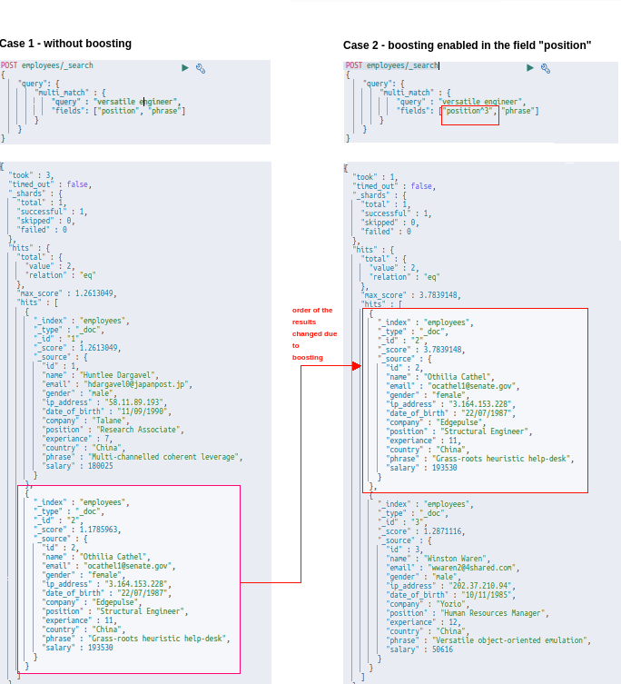
3. Boosting
While querying, it is often helpful to get the more favored results first. The simplest way of doing this is called boosting in Elasticsearch. And this comes in handy when we query multiple fields. For example, consider the following query:
POST employees/_search
{
    "query": {
        "multi_match" : {
            "query" : "versatile Engineer",
            "fields": ["position^3", "phrase"]
        }
    }
}
This will return the response with the documents matching the “position” field to be in the top rather than with that of the field “phrase”.
4. Sorting
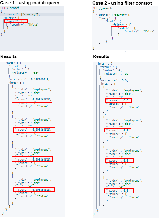
4.1 Default Sorting
When there is no sort parameter specified in the search request, Elasticsearch returns the document based on the descending values of the “_score” field. This “_score” is computed by how well the query has matched using the default scoring methodologies of Elasticsearch. In all the examples we have discussed above you can see the same behavior in the results.
It is only when we use the “filter” context that there is no scoring computed, so as to make the return of the results faster.
4.2 How to Sort by a Field
Elasticsearch gives us the option to sort on the basis of a field. Say, let us need to sort the employees based on their descending order of experience. We can use the below query with the sort option enabled to achieve that:
GET employees/_search
{
   "_source": ["name","experience","salary"],
  "sort": [
    {
      "experience": {
        "order": "desc"
      }
    }
  ]

}
The results of the above query is given below:
"hits" : [
      {
        "_index" : "employees",
        "_type" : "_doc",
        "_id" : "3",
        "_score" : null,
        "_source" : {
          "name" : "Winston Waren",
          "experience" : 12,
          "salary" : 50616
        },
        "sort" : [
          12
        ]
      },
      {
        "_index" : "employees",
        "_type" : "_doc",
        "_id" : "4",
        "_score" : null,
        "_source" : {
          "name" : "Alan Thomas",
          "experience" : 12,
          "salary" : 300000
        },
        "sort" : [
          12
        ]
      },
      {
        "_index" : "employees",
        "_type" : "_doc",
        "_id" : "2",
        "_score" : null,
        "_source" : {
          "name" : "Othilia Cathel",
          "experience" : 11,
          "salary" : 193530
        },
        "sort" : [
          11
        ]
      },
      {
        "_index" : "employees",
        "_type" : "_doc",
        "_id" : "1",
        "_score" : null,
        "_source" : {
          "name" : "Huntlee Dargavel",
          "experience" : 7,
          "salary" : 180025
        },
        "sort" : [
          7
        ]
      }
    ]
As you can see from the above response, the results are ordered based on the descending values of the employee experience. Also, there are two employees, with the same experience level as 12.
4.3 How to Sort by Multiple Fields
In the above example, we saw that there are two employees with the same experience level of 12, but we need to sort again based on the descending order of the salary. We can provide multiple fields for sorting too, as shown in the query demonstrated below:
GET employees/_search
{
  "_source": [
    "name",
    "experience",
    "salary"
  ],
  "sort": [
    {
      "experience": {
        "order": "desc"
      }
    },
    {
      "salary": {
        "order": "desc"
      }
    }
  ]
}
Now we get the below results:
"hits" : [
      {
        "_index" : "employees",
        "_type" : "_doc",
        "_id" : "4",
        "_score" : null,
        "_source" : {
          "name" : "Alan Thomas",
          "experience" : 12,
          "salary" : 300000
        },
        "sort" : [
          12,
          300000
        ]
      },
      {
        "_index" : "employees",
        "_type" : "_doc",
        "_id" : "3",
        "_score" : null,
        "_source" : {
          "name" : "Winston Waren",
          "experience" : 12,
          "salary" : 50616
        },
        "sort" : [
          12,
          50616
        ]
      },
      {
        "_index" : "employees",
        "_type" : "_doc",
        "_id" : "2",
        "_score" : null,
        "_source" : {
          "name" : "Othilia Cathel",
          "experience" : 11,
          "salary" : 193530
        },
        "sort" : [
          11,
          193530
        ]
      },
      {
        "_index" : "employees",
        "_type" : "_doc",
        "_id" : "1",
        "_score" : null,
        "_source" : {
          "name" : "Huntlee Dargavel",
          "experience" : 7,
          "salary" : 180025
        },
        "sort" : [
          7,
          180025
        ]
      }
    ]
In the above results, you can see that within the employees having same experience levels, the one with the highest salary was promoted early in the order (Alan and Winston had same experience levels, but unlike the previous search results, here Alan was promoted as he had higher salary).
Note: If we change the order of sort parameters in the sorted array, that is if we keep the “salary” parameter first and then the “experience” parameter, then the search results would also change. The results will first be sorted on the basis of the salary parameter and then the experience parameter will be considered, without impacting the salary-based sorting.
Let us invert the order of sort of the above query, that is “salary” is kept first and the “experience” as shown below:
GET employees/_search
{
  "_source": [
    "name",
    "experience",
    "salary"
  ],
  "sort": [
    {
      "salary": {
        "order": "desc"
      }
    },
    {
      "experience": {
        "order": "desc"
      }
    }
  ]
}
The results would be like below:
"hits" : [
      {
        "_index" : "employees",
        "_type" : "_doc",
        "_id" : "4",
        "_score" : null,
        "_source" : {
          "name" : "Alan Thomas",
          "experience" : 12,
          "salary" : 300000
        },
        "sort" : [
          300000,
          12
        ]
      },
      {
        "_index" : "employees",
        "_type" : "_doc",
        "_id" : "2",
        "_score" : null,
        "_source" : {
          "name" : "Othilia Cathel",
          "experience" : 11,
          "salary" : 193530
        },
        "sort" : [
          193530,
          11
        ]
      },
      {
        "_index" : "employees",
        "_type" : "_doc",
        "_id" : "1",
        "_score" : null,
        "_source" : {
          "name" : "Huntlee Dargavel",
          "experience" : 7,
          "salary" : 180025
        },
        "sort" : [
          180025,
          7
        ]
      },
      {
        "_index" : "employees",
        "_type" : "_doc",
        "_id" : "3",
        "_score" : null,
        "_source" : {
          "name" : "Winston Waren",
          "experience" : 12,
          "salary" : 50616
        },
        "sort" : [
          50616,
          12
        ]
      }
    ]
You can see that the candidate with experience value 12 came below the candidate with experience value 7, as the latter had more salary than the former.
5. Compound Queries
So far, in the tutorial, we have seen that we fired single queries, like finding a text match or finding the age ranges, etc. But more often in the real world, we need multiple conditions to be checked and documents to be returned based on that. Also, we might need to modify the relevance or score parameter of the queries or to change the behavior of the individual queries, etc. Compound queries are the queries that help us to achieve the above scenarios. In this section, let us have a look into a few of the most helpful compound queries.
5.1. The Bool Query
Bool query provides a way to combine multiple queries in a boolean manner. That is for example if we want to retrieve all the documents with the keyword “researcher” in the field “position” and those who have more than 12 years of experience we need to use the combination of the match query and that of the range query. This kind of query can be formulated using the bool query. The bool query has mainly 4 types of occurrences defined:
| must | The conditions or queries in this must occur in the documents to consider them a match. Also, this contributes to the score value. For example, if we keep query A and query B in the must section, each document in the result would satisfy both the queries, i.e. query A AND query B |
| should | The conditions/queries should match. Result = query A OR query B |
| filter | Conditions are the same as the must clause, but no score will be calculated. |
| must_not | The conditions/queries specified must not occur in the documents. Scoring is ignored and kept as 0 as the results are ignored. |
A typical bool query structure would be like the below:
POST _search
{
  "query": {
    "bool" : {
      "must" : [],
      "filter": [],
      "must_not" : [],
      "should" : []
    }
  }
}
Now let’s explore how we can use the bool query for different use cases.
Bool Query Example 1 – Must
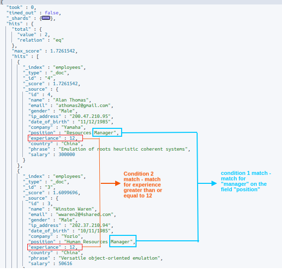
In our example, let us say, we need to find all employees who have 12 years of experience or more AND also have the word “manager” in the “position” field. We can do that with the following bool query
POST employees/_search
{
  "query": {
    "bool": {
      "must": [
        {
          "match": {
            "position": "manager"
          }
        },
        {
          "range": {
            "experience": {
              "gte": 12
            }
          }
        }
      ]
    }
  }
}
The response for the above query will have documents matching both the queries in the “must” array and is shown below:
Bool Query Example 2 – Filter
The previous example demonstrated the “must” parameter in the bool query. You can see in the results of the previous example that the results had values in the “_score” field. Now let us use the same query, but this time let us replace the “must” with “filter” and see what happens:
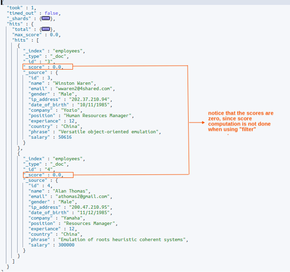
From the above screenshot, it can be seen that the score value is zero for the search results. This is because when using the filter context, the score is not computed by Elasticsearch in order to make the search faster.
If we use a must condition with a filter condition, the scores are calculated for the clauses in must, but no scores are computed for the filter side.
Bool Query Example 3 – Should
Now, let us see the effect of the “should” section in the bool query. Let us add a should clause in the above example’s query. This “should” condition is to match documents that contain the text “versatile” in the “phrase” fields of the documents. The query for this would look like below:
POST employees/_search
{
  "query": {
    "bool": {
      "must": [
        {
          "match": {
            "position": "manager"
          }
        },
        {
          "range": {
            "experience": {
              "gte": 12
            }
          }
        }
      ],
    "should": [
      {
        "match": {
          "phrase": "versatile"
        }
      }
    ]
    }
  }
}
Now the results will be the same 2 documents that we received in the previous example, but the document with id=3, which was shown as the last result is shown as the first result. This is because the clause in the “should” array is occurring in that document and hence the score has increased, and so it was promoted as the first document.

Bool Query Example 4 – Multiple Conditions
A real-world example of a bool query might be more complex than the above simple ones. What if users want to get employees who might be from the companies “Yamaha” or “Telane”, and are of the title “manager” or “associate”, with a salary greater than 100,000?
The above-stated condition, when put in short can be shortened as below
(company = Yamaha OR company = Yozio ) AND (position = manager OR position = associate ) AND (salary>=100000)This can be achieved using multiple bool queries inside a single must clause, as shown in the below query:
POST employees/_search
{
    "query": {
        "bool": {
            "must": [
              {
                "bool": {
                    "should": [{
                        "match": {
                            "company": "Talane"
                        }
                    }, {
                        "match": {
                            "company": "Yamaha"
                        }
                    }]
                }
            },
            {
                "bool": {
                    "should": [
                      {
                        "match": {
                            "position": "manager"
                        }
                    }, {
                        "match": {
                            "position": "Associate"
                        }
                    }
                    ]
                }
            }, {
                "bool": {
                    "must": [
                      {
                        "range": {
                          "salary": {
                            "gte": 100000
                          }
                        }
                      }
                      ]
                }
            }]
        }
    }
}
5.2. Boosting Queries
Sometimes, there are requirements in the search criteria where we need to demote certain search results but do not want to omit them from the search results altogether. In such cases, boosting the query would become handy. Let us go through a simple example to demonstrate this.
Let us search for all the employees from China and then demote the employees from the company “Telane” in search results. We can use the boosting query like the below:
POST  employees/_search
{
    "query": {
        "boosting" : {
            "positive" : {
                "match": {
                  "country": "china"
                }
            },
            "negative" : {
                 "match": {
                  "company": "Talane"
                }
            },
            "negative_boost" : 0.5
        }
    }
}
Now the response of the above query would be as given below, where you can see that the employee of the company “Talane” is ranked the last and has a difference of 0.5 in score with the previous result.
We can apply any query to the “positive” and “negative” sections of the boosting query. This is good when applying multiple conditions with a bool query. An example of such a query is given below:
GET employees/_search
{
  "query": {
    "boosting": {
      "positive": {
        "bool": {
          "should": [
            {
              "match": {
                "country": {
                  "query": "china"
                }
              }
            },
            {
              "range": {
                "experience": {
                  "gte": 10
                }
              }
            }
          ]
        }
      },
      "negative": {
        "match": {
          "gender": "female"
        }
      },
      "negative_boost": 0.5
    }
  }
}
5.3 Function Score Queries
The function_score query enables us to change the score of the documents that are returned by a query. The function_score query requires a query and one or more functions to compute the score. If no functions are mentioned, the query is executed as normal.
The most simple case of the function score, without any function, is demonstrated below:

5.3.1 function_score: weight
As said in the earlier sections, we can use one or more score functions in the “functions” array of the “function_score” query. One of the simplest yet important functions is the “weight” score function.
According to the documentation, the weight score allows you to multiply the score by the provided weight. The weight can be defined per function in the functions array (example above) multiplied by the score computed by the respective function.
Let us demonstrate the example using a simple modification of the above query. Let us include two filters in the “functions” part of the query. The first one would search for the term “coherent” in the “phrase” field of the document and, if found, will boost the score by a weight of 2. The second clause would search for the term “emulation” in the field “phrase” and will boost by a factor of 10 for such documents. Here is the query:
GET employees/_search
{
"_source": ["position","phrase"],
  "query": {
    "function_score": {
      "query": {
        "match": {
          "position": "manager"
        }
      },
      "functions": [
        {
          "filter": {
            "match": {
              "phrase": "coherent"
            }
          },
          "weight": 2
        },
        {
          "filter": {
            "match": {
              "phrase": "emulation"
            }
          },
          "weight": 10
        }
      ],
      "score_mode": "multiply",
      "boost": "5",
      "boost_mode": "multiply"
    }
  }
}
The response of the above query is as below:
{
  "took" : 0,
  "timed_out" : false,
  "_shards" : {
    "total" : 1,
    "successful" : 1,
    "skipped" : 0,
    "failed" : 0
  },
  "hits" : {
    "total" : {
      "value" : 2,
      "relation" : "eq"
    },
    "max_score" : 72.61542,
    "hits" : [
      {
        "_index" : "employees",
        "_type" : "_doc",
        "_id" : "4",
        "_score" : 72.61542,
        "_source" : {
          "phrase" : "Emulation of roots heuristic coherent systems",
          "position" : "Resources Manager"
        }
      },
      {
        "_index" : "employees",
        "_type" : "_doc",
        "_id" : "3",
        "_score" : 30.498476,
        "_source" : {
          "phrase" : "Versatile object-oriented emulation",
          "position" : "Human Resources Manager"
        }
      }
    ]
  }
}
The simple match part of the query on the position field yielded a score of 3.63 and 3.04 respectively for the two documents. When the first function in the functions array was applied (match for the “coherent” keyword), there was only one match, and that was for the document with id = 4.
The current score of that document was multiplied by the weight factor for the match “coherent,” which is 2. Now the new score for the document becomes 3.63*2 = 7.2
After that, the second condition (match for “emulation”) matched for both documents.
So the current score of the document with id=4 is 7.2*10 = 72, where 10 is the weight factor for the second clause.
The document with id=3 matched only for the second clause and hence its score = 3.0*10 = 30.
5.3.2 function_score: script_score
It often occurs that we need to compute the score based on one or more fields/fields; for that, the default scoring mechanism is insufficient. Elasticsearch provides us with the “script_score” score function to compute the score based on custom requirements. Here, we can provide a script that will return the score for each document based on the custom logic on the fields.
Say, for example, we need to compute the scores as a function of salary and experience, i.e. the employees with the highest salary-to-experience ratio should score more. We can use the following function_score query for the same:
GET employees/_search
{
  "_source": [
    "name",
    "experience",
    "salary"
  ],
  "query": {
    "function_score": {
      "query": {
        "match_all": {}
      },
      "functions": [
        {
          "script_score": {
            "script": {
              "source": "(doc['salary'].value/doc['experience'].value)/1000"
            }
          }
        }
      ],
      "boost_mode": "replace"
    }
  }
}
In the above query, the script part written in Painless is:
(doc[‘salary’].value/doc[‘experience’].value)/1000
The script above will generate the scores for the search results. For example, for an employee with a salary = 180025 and experience = 7, the score generated would be:
(180025/7)/1000 = 25
Since we are using the boost_mode: replace the scores computed by a script that is placed precisely as the score for each document. The results for the above query are given in the screenshot below:

5.3.3 function_score: field_value_factor
We can use a field from the document to influence the score by using the “field_value_factor” function. This is, in some ways, a simple alternative to “script_score.” In our example, we make use of the “experience” field value to influence our score as below
GET employees/_search
{
  "_source": ["name","experience"],
    "query": {
        "function_score": {
            "field_value_factor": {
                "field": "experience",
                 "factor": 0.5,
                "modifier": "square",
                "missing": 1
            }
        }
    }
}
The response for the above query is as shown below:
{
  "took" : 0,
  "timed_out" : false,
  "_shards" : {
    "total" : 1,
    "successful" : 1,
    "skipped" : 0,
    "failed" : 0
  },
  "hits" : {
    "total" : {
      "value" : 4,
      "relation" : "eq"
    },
    "max_score" : 36.0,
    "hits" : [
      {
        "_index" : "employees",
        "_type" : "_doc",
        "_id" : "3",
        "_score" : 36.0,
        "_source" : {
          "name" : "Winston Waren",
          "experience" : 12
        }
      },
      {
        "_index" : "employees",
        "_type" : "_doc",
        "_id" : "4",
        "_score" : 36.0,
        "_source" : {
          "name" : "Alan Thomas",
          "experience" : 12
        }
      },
      {
        "_index" : "employees",
        "_type" : "_doc",
        "_id" : "2",
        "_score" : 30.25,
        "_source" : {
          "name" : "Othilia Cathel",
          "experience" : 11
        }
      },
      {
        "_index" : "employees",
        "_type" : "_doc",
        "_id" : "1",
        "_score" : 12.25,
        "_source" : {
          "name" : "Huntlee Dargavel",
          "experience" : 7
        }
      }
    ]
  }
}
The score computation for the above would be like below:
Square of (factor*doc[experience].value)
For a document with “experience” containing the value of 12, the score will be:
square of (0.5*12) = square of (6) = 36
5.3.4 function_score: Decay Functions
Consider the use case of searching for hotels near a location. For this use case, the nearer the hotel is, the more relevant the search results are, but when it is farther away, the search becomes insignificant. Or, to refine it further, if the hotel is farther than a walkable distance of 1km from the location, the search results should show a rapid decline in the score. Whereas the ones inside the 1km radius should be scored higher.
For this kind of use case, a decaying scoring mode is the best choice, i.e., the score will start to decay from the point of interest. We have score functions in Elasticsearch for this purpose called the decay functions. There are three types of decay functions, namely “gauss,” “linear,” and “exponential” or “exp.”
Let us make an example of a use case from our data. We need to score the employees based on their salaries. The ones near 200000 and between the ranges 170000 to 230000 should get higher scores, and the ones below and above the range should have significantly lower scores.
GET employees/_search
{
  "_source": [
    "name",
    "salary"
  ],
  "query": {
    "function_score": {
      "query": {
        "match_all": {}
      },
      "functions": [
       {
         "gauss": {
           "salary": {
             "origin": 200000,
             "scale": 30000
           }
         }
       }
      ],
      "boost_mode": "replace"
    }
  }
}
Here the ‘origin’ represents the point to start calculating the distance. The scale represents the distance from the origin, up to which the priority should be given for scoring. There are additional parameters that are optional and can be viewed in Elastic’s documentation
The above query results are shown in the image below:

6. Parent-Child Queries
One-to-many relationships can be handled using the parent-child method (now called the join operation) in Elasticsearch. Let us demonstrate this with an example scenario. Consider we have a forum where anyone can post any topic (say posts). Users can comment on individual posts. So in this scenario, we can consider the individual posts as the parent documents and the comments to them as their children. This is best explained in the below figure:

For this operation, we will have a separate index created, with special mapping (schema) applied.
Create the index with join data type with the below request
PUT post-comments
{
  "mappings": {
    "properties": {
      "document_type": {
        "type": "join",
        "relations": {
          "post": "comment"
        }
      }
    }
  }
}
In the above schema, you can see there is a type named “join”, which indicates, that this index is going to have parent-child-related documents. Also, the ‘relations’ object has the names of the parent and child identifiers defined.
That is “post” and “comment” refer to parent and child roles respectively. Each document will consist of a field named “document_type” which will have the value “post” or “comment”. The value “post” will indicate that the document is a parent and the value “comment” will indicate the document is a “child”.
Let us index some documents for this:
PUT post-comments/_doc/1
{
"document_type": {
    "name": "post"
  },
"post_title" : "Angel Has Fallen"
}
PUT post-comments/_doc/2
{
"document_type": {
    "name": "post"
  },
"post_title" : "Beauty and the beast - a nice movie"
}
Indexing child documents for the document with id=1
PUT post-comments/_doc/A?routing=1
{
"document_type": {
    "name": "comment",
    "parent": "1"
  },
"comment_author": "Neil Soans",
"comment_description": "'Angel has Fallen' has some redeeming qualities, but they're too few and far in between to justify its existence"
}
PUT post-comments/_doc/B?routing=1
{
"document_type": {
    "name": "comment",
    "parent": "1"
  },
"comment_author": "Exiled Universe",
"comment_description": "Best in the trilogy! This movie wasn't better than the Rambo movie, but it was very very close."
}
Indexing child documents for the document with id=2
PUT post-comments/_doc/D?routing=2
{
"document_type": {
    "name": "comment",
    "parent": "2"
  },
"comment_author": "Emma Cochrane",
"comment_description": "There's the sublime beauty of a forgotten world and the promise of happily-ever-after to draw you to one of your favourite fairy tales, once again. Give it an encore."
}
PUT post-comments/_doc/E?routing=2
{
"document_type": {
    "name": "comment",
    "parent": "2"
  },
"comment_author": "Common Sense Media Editors",
"comment_description": "Stellar music, brisk storytelling, delightful animation, and compelling characters make this both a great animated feature for kids and a great movie for anyone"
}
Before getting into followup queries that can be done with joined fields, it is important to note that these types of queries can add significant processing and delays to query performance and may trigger global ordinal creation. These should only be used in one-to-many relationships where the child entities greatly outnumber the parents.
6.1 The has_child Query
This will query the child’s documents and then return the parents associated with them as the results. Suppose we need to query for the term “music” in the field “comment_description” in the child documents and to get the parent documents corresponding to the search results, we can use the has_child query as below:
GET post-comments/_search
{
  "query": {
    "has_child": {
      "type": "comment",
      "query": {
        "match": {
          "comment_description": "music"
        }
      }
    }
  }
}
For the above query, the child documents that matched the search was only the document with id=E, for which the parent is the document with id=2. The search result would get us the parent document as below:

6.2 The has_parent Query
The has_parent query performs the opposite of the has_child query, that is it will return the child documents of the parent documents that matched the query.
Let us search for the word “Beauty” in the parent document and return the child documents for the matched parents. We can use the below query for that
GET post-comments/_search
{
  "query": {
    "has_parent": {
      "parent_type": "post",
      "query": {
        "match": {
          "post_title": "Beauty"
        }
      }
    }
  }
}
The matched parent document for the above query is the one with document id =1. As you can see from the response below, the children’s documents corresponding to the id=1 document are returned by the above query:

6.3 Fetching Child Documents with Parents
Sometimes, we require both the parent and child documents in the search results. For example, if we are listing the posts, it would also be nice to display a few comments below it as it would be more eye candy.
Elasticsearch allows the same. Let us use the has_child query to return parents and this time, we will fetch the corresponding child documents too.
The following query contains a parameter called “inner_hits” which will allow us to do the exact same.
GET post-comments/_search
{
  "query": {
    "has_child": {
      "type": "comment",
      "query": {
        "match": {
          "comment_description": "music"
        }
      },
      "inner_hits": {}
    }
  }
}

7. Other Query Examples
7.1 The query_string Query
The “query_string” query is a special multi-purpose query, which can combine the usage of several other queries like “match”, ”multi-match”, “wildcard”, “regexp”, etc. The “query_string” query follows a strict format and the violation of it would output error messages. Hence, even with its capabilities, it is seldom used for the implementation of user-facing search boxes.
Let us see a sample query in action:
POST employees/_search
{
  "query": {
    "query_string": {
      "query": "(roots heuristic systems) OR (enigneer~) OR (salary:(>=10000 AND <=52000)) ",
      "fields": [
        "position",
        "phrase^3"
      ]
    }
  }
}
The above query will search for the words “roots” OR “heuristic” OR “systems” OR “engineer” (the usage of ~ in the query indicates the usage of a fuzzy query) in the fields “position” and “phrase” and return the results. “phrase^3” indicates the matches found on the field “phrase” should be boosted by a factor of 3. The salary:(>10000 AND <=52000), indicates to fetch the documents which have the value of the field “salary”, falling between 10000 and 52000.
7.2 The simple_query_string query
The “simple_query_string” query is a simplified form of the query_string query with two major differences: first, it is more fault-tolerant, which means it does not return errors if the syntax is wrong. Rather, it ignores the faulty part of the query. This makes it more friendly for user interface search boxes. Second, the operators AND/OR/NOT are replaced with +/|/-
A simple example of the query would be:
POST employees/_search
{
  "query": {
    "simple_query_string": {
      "query": "(roots) | (resources manager) + (male) ",
      "fields": [
        "gender",
        "position",
        "phrase^3"
      ]
    }
  }
}
The above query would search for “roots” OR “resources” OR “manager” AND “male” in all of the fields mentioned in the “fields” array.
7.3 Named Queries
Named queries, as the name suggests, are all about the naming of queries. There are scenarios when it helps us to identify which part/parts of the query matched the document. Elasticsearch provides us with that exact feature by allowing us to name the query or parts of the query so as to see these names with the matching documents.
Let us see this in action, with the below example in the image:
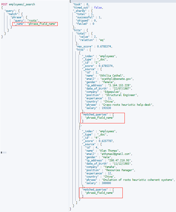
In the above example, the match query is supplied with a “_name” parameter, which has the name for the query as “phrase_field_name”. In the results, we have documents that matched the results coming with an array field named “matched_queries” which has the names of the matched query/query (here “phrase_field_name”).
The below example shows the usage of the named queries in a bool query, which is one of the most common use cases of the named queries.

With these Elasticsearch queries users can get powerful insights from their data. The ELK stack and a well-written query can provide users with tools to improve insights into other stacks. The ELK stack is commonly used to store and search observability data, logs, as well as custom documents. For example, if you need help enhancing Kubernetes logging, Elasticsearch can help store data that is easily lost in Kubernetes.
Want to get all the power of ELK without the hidden ELK stack cost? Take Coralogix for a 14-day free test drive and see the difference