grafana Archives

Grafana Loki: Open Source Log Aggregation Inspired by Prometheus

Posted on May 19, 2021June 19, 2025 by eugene evdokimov

Logging solutions are a must-have for any company with software systems. They are necessary to monitor your software solution’s health, prevent issues before they happen, and troubleshoot existing problems.

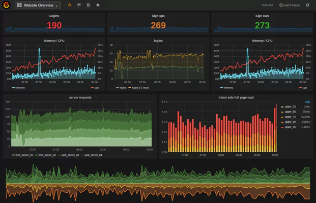
The market has many solutions which all focus on different aspects of the log monitoring problem. These solutions include both open source and proprietary software and tools built into cloud provider platforms, and give a variety of different features to meet your specific needs. Grafana Loki is a relatively new industry solution so let’s take a closer look at what it is, where it came from, and if it might meet your logging needs.

What is Grafana Loki, and Where Did it Come From?

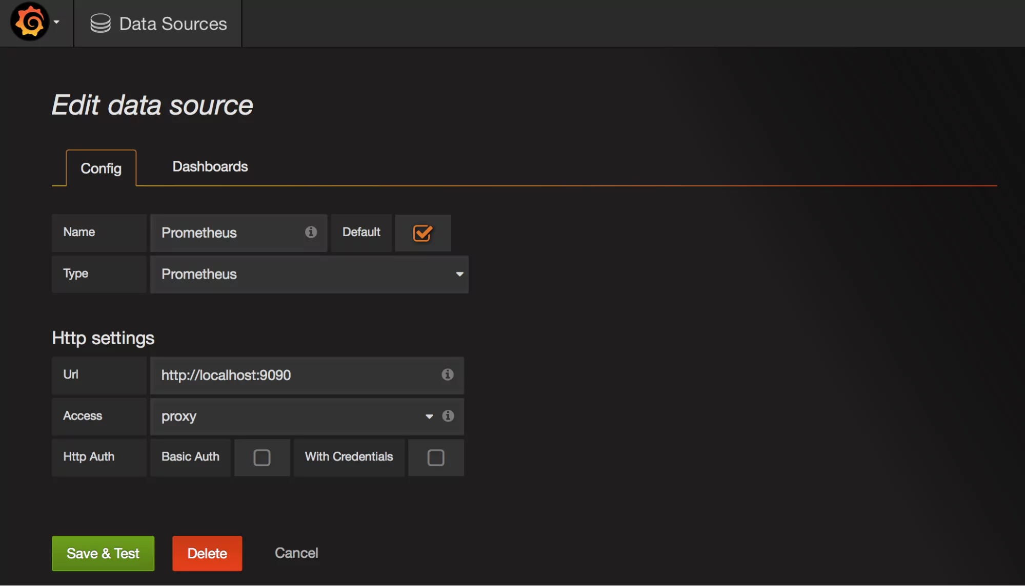
Grafana Loki based its architecture on Prometheus’s use of labels to index data. Doing this allows Loki to store indexes in less space. Further, Loki’s design directly plugs into Prometheus, meaning developers can use the same label criteria with both tools.

Prometheus is open source and has become the defacto standard for time-series metrics monitoring solutions. Being a cloud-native solution, developers primarily use Prometheus when software is built with Kubernetes or other cloud-native solutions.

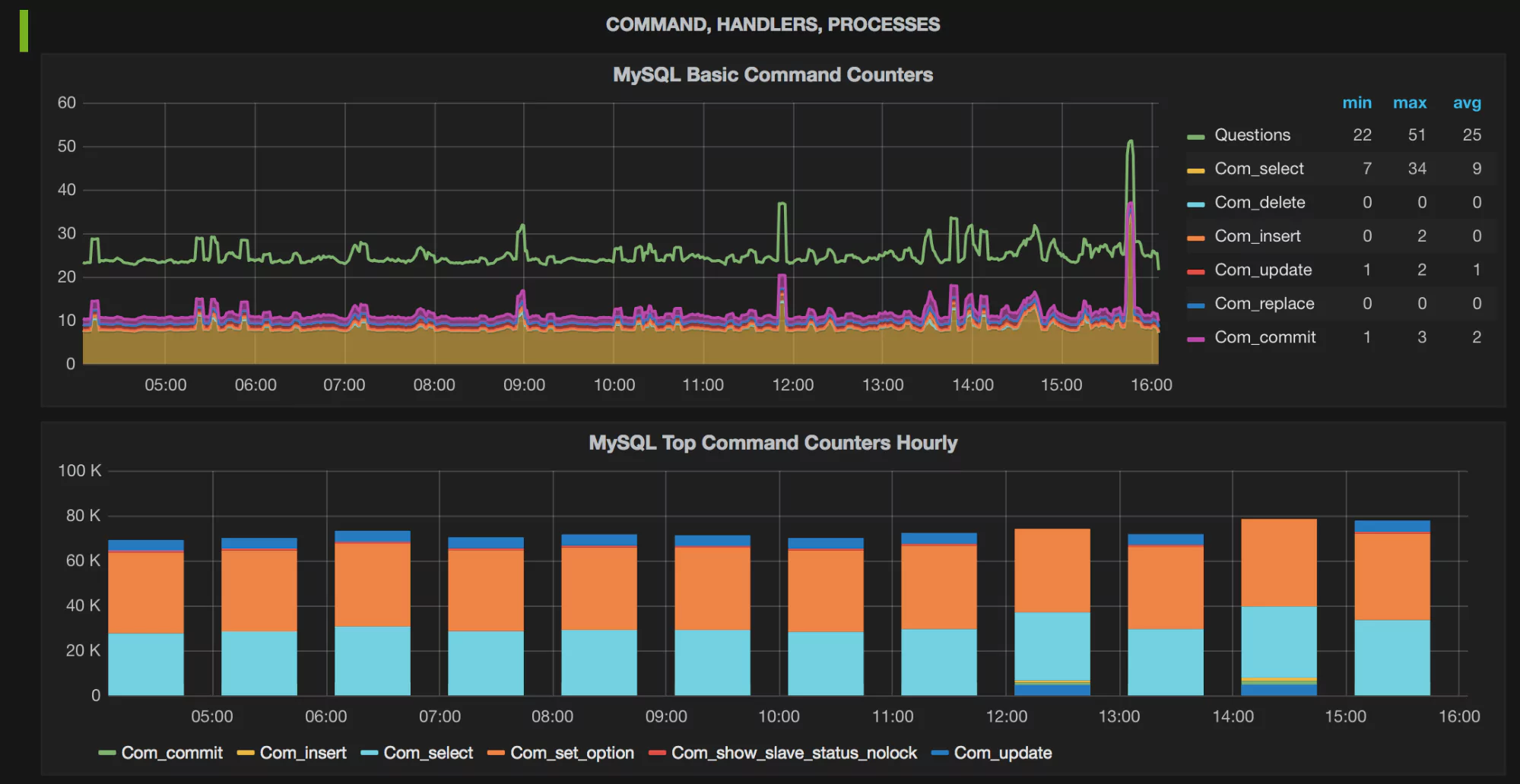
Prometheus is unique in its capabilities of collecting multi-dimensional data from multiple sources, making it an attractive solution for companies running microservices on the cloud. It has an alerting system for metrics, but developers often augment it with other logging solutions. Other logging solutions tend to give more observability into software systems and add a visualization component to the logs.

Prometheus created a new query language (PromQL), making it challenging to visualize logging for troubleshooting and monitoring. Many of the available logging solutions were built before Prometheus came to the logging scene in 2012 and did not support linking to Prometheus.

What Need does Grafana Loki Fill?

Grafana Loki was born out of a desire to have an open source tool that could quickly select and search time-series logs where the logs are stored stably. Discerning system issues may include log visualization tools with a querying ability, log aggregation, and distributed log tracing.

Existing open source tools do not easily plug into Prometheus for troubleshooting. They did not allow developers to search for Prometheus’s metadata for a specific period, instead only allowing them to search the most recent logs this way. Further, log storage was not efficient, so developers could quickly max out their logging limits and need to consider which logs they could potentially live without. With some tools, crashes could mean that logs are lost forever.

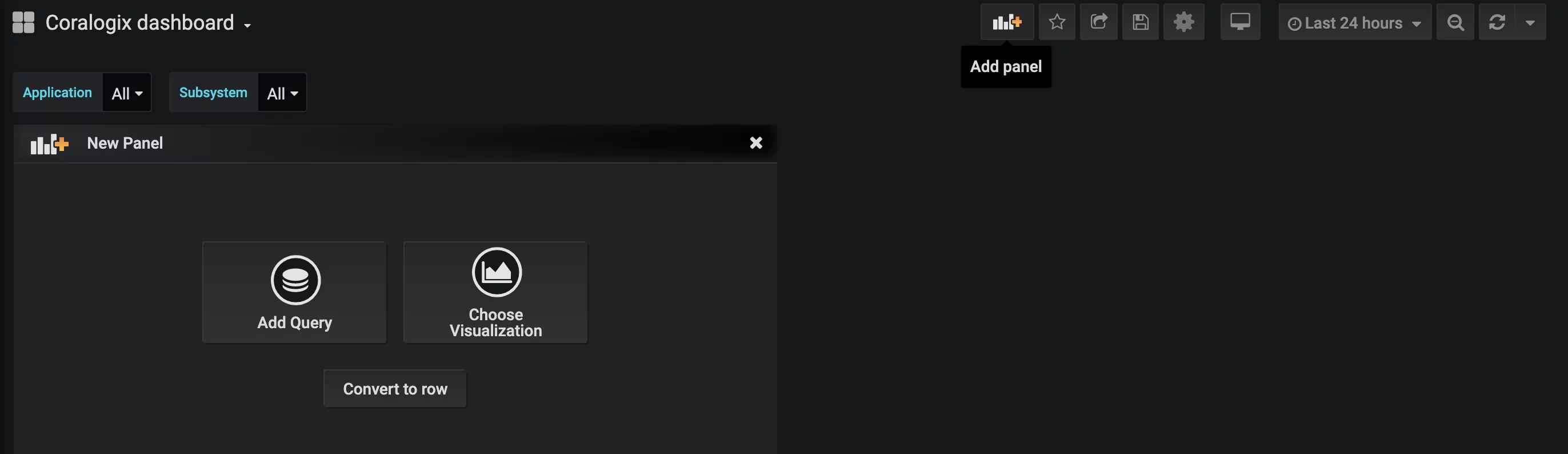
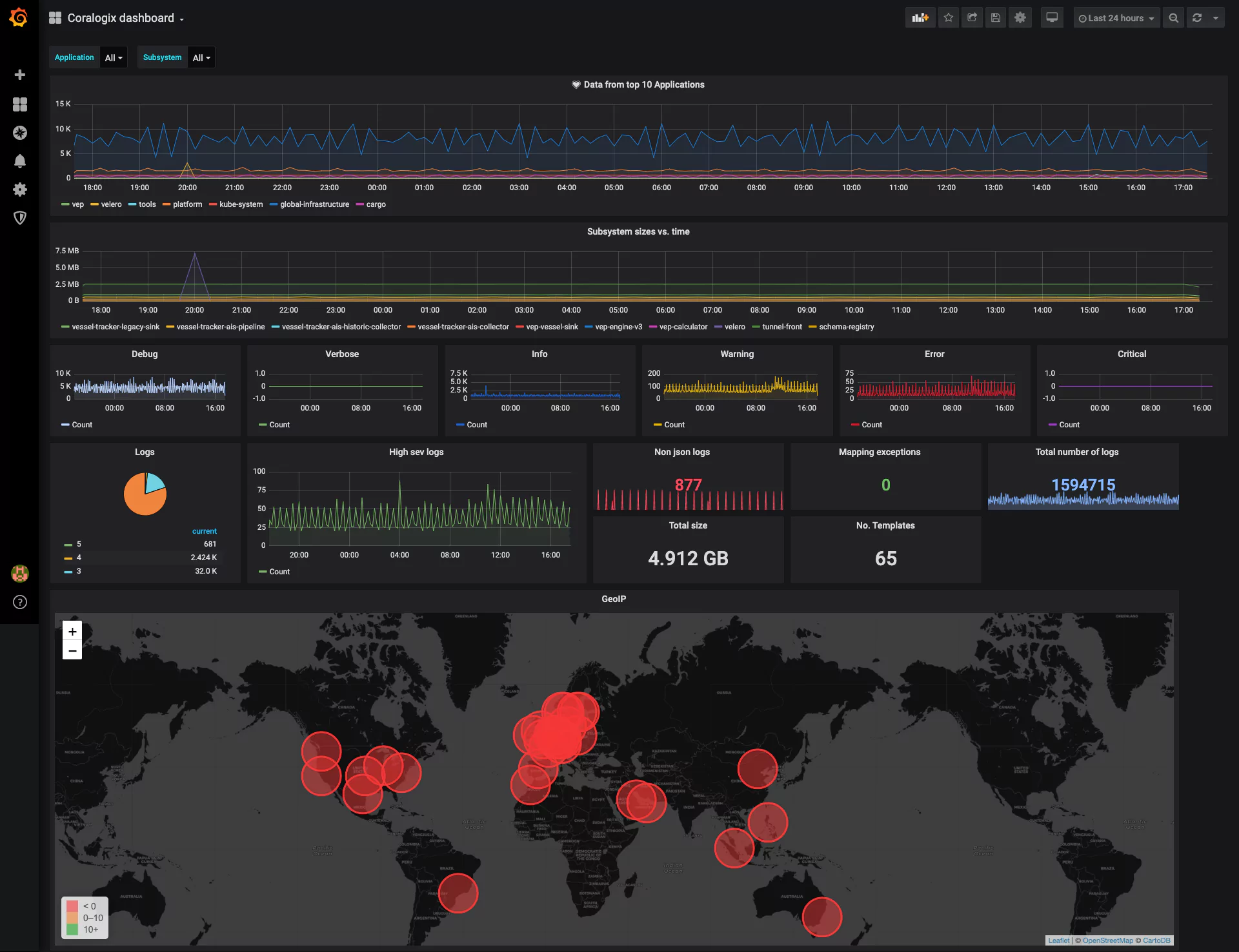
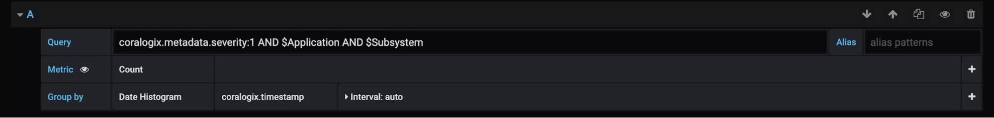
It’s important to note that there are proprietary tools on the market that do not have these same limitations and have capabilities far beyond what open source tools are capable of providing. These tools can allow for time-bound searching, log aggregation, and distributed tracing with a single tool instead of using a separate open source tool for each need. Coralogix, for example, allows querying of logs using SQL queries or Kibana visualizations and also ingests Prometheus metrics along with metrics from several other sources.

Grafana Loki’s Architecture

Built from Components

Developers built Loki’s service from a set of components (or modules). There are four components available for use: distributor, ingester, querier, and query frontend.

Distributor

The distributor module handles and validates incoming data streams from clients. Valid data is chunked and sent to multiple ingesters for parallel processing.

The distributor relies on Prometheus-like labels to validate log data in the distributor and to process in different downstream modules. Without labels, Grafana Loki cannot create the index it requires for searching. Suppose your logs do not have appropriate labels, for example. In that case, if you are loading from services other than Prometheus, the Loki architecture may not be the optimal choice for log aggregations.

Ingester

The ingester module writes data to long-term storage. Loki does not store the log data it ingests, instead only indexing metadata. The object storage used is configurable, for example, AWS S3, Apache Cassandra, or local file systems.

The ingester also returns data for in-memory queries. Ingester crashes cause unflushed data to be lost. Loki can irretrievably lose logs from ingesters with improper user setup ensuring redundancy.

Querier

Grafana Loki uses the querier module to handle the user’s queries on the ingester and the object stores. Queries are run first against local storage and then against long-term storage. The querier must handle duplicate data because it queries multiple places, and the ingesters do not detect duplicate logs in the writing process. The querier has an internal mechanism, so it returns data with the same timestamp, label data, and log data only once.

Query Frontend

The query frontend module optionally gives API endpoints for queries that enable parallelization of large queries. The query frontend still uses queries, but it will split a large query into smaller ones and execute the reads on logs in parallel. This ability is helpful if you are testing out Grafana Loki and do not yet want to set up a querier in detail.

Object Stores

Loki needs long-term data storage for holding queryable logs. Grafana Loki requires an object store to hold both compressed chunks written by the ingester and the key-value pairs for the chunk data. Fetching data from long-term storage can take more time than local searches.

The file system is the only no-added-cost option available for storing your chunked logs, with all others belonging to managed object stores. The file system comes with downsides since it is not scalable, not durable, and not highly available. It’s recommended to use the file system storage for testing or development only, not for troubleshooting in production environments.

There are many other log storage options available that are scalable, durable, and highly available. These storage solutions accrue costs for reading and writing data and data storage. Coralogix, a proprietary observability platform, analyzes data immediately after ingestion (before indexing and storage) and then charges based on how the data will be used. This kind of pricing model reduces hidden or unforeseen costs that are often associated with Cloud storage models.

Grafana Loki’s Feature Set

Horizontally Scalable

Developers can run Loki in one of two modes depending on the target value. When developers set the target to all, Loki runs components on a single server in monolith mode. Setting the target to one of the available component names runs Loki in a horizontally-scalable or microservices mode where a server is available for each component.

Users can scale distributors, ingestors, and querier components as needed to handle the size of their stored logs and the speed of responses.

Inexpensive Log Storage and Querying

Being open source, Grafana Loki is an inexpensive option for log analytics. The cost involved with using the free-tier cloud solution, or the source code installed through Tanka or Docker, is in storing the log and label data.

Loki recommends labels be kept as small as possible to keep querying fast. As a result, label stores can be relatively small compared to the complete log data. Complete logs are compressed with your choice of the tool before being stored, making the storage even more efficient.

Note: Compression tools generally have a tradeoff between storage size and read speed, meaning developers will need to consider cost versus speed when setting up their Loki system.

Grafana uses Cloud storage solutions like AWS S3 or Google’s GCS. Loki’s cost depends on the size of logs needed for analysis and the frequency of read/write operations. For example, AWS S3 charges for each GB stored and for each request made against the S3 bucket.

Fast Querying

When logs are imported into Grafana Loki using Promtail, ingesters split out labels from the log data. Labels should be as limited as possible since they are used to select logs searched during queries. An implicit requirement of getting speedy queries with Loki is concise and limited labels.

When you query, Loki splits data according to time and then sharded by the index. Available queriers are then applied to read the shard’s entire contents looking for the given search parameters. The more queriers available and the smaller the index, the faster the query response will be available.

Grafana Loki uses brute force along with parallelized components to gain speed of querying. This speed gained with Grafana Loki is considerable for a brute force methodology. Loki uses this brute-force method to gain simplicity over fully indexed solutions. However, fully indexed solutions can search logs more robustly.

Open Source

Open source solutions like Grafana Loki always have drawbacks. The Loki team has had a great interest in their product and works diligently to address the new platform’s issues. Grafana Loki relies on community assistance with documentation and features. Community reliance means setting up and enhancing a log analytics platform with Loki can take significant and unexpected developer resources.

To ensure speedy responses, users must sign up for Enterprise services which come at a cost like other proprietary systems. If you are considering these Enterprise services, ensure you have looked at other proprietary solutions, so you get the most valuable features from your log analytics platform.

Summary

Grafana Loki is an open source, horizontally scalable, brute-force log aggregation tool built for use with Prometheus. Production users will need to combine Loki with a cloud account for log storage.

Loki gives users a low barrier-to-entry tool that plugs into both Prometheus for metrics and Grafana for log visualization in a simple way. The free version does have drawbacks since it is not guaranteed to be available. There are also instances where Loki can lose logs without proper redundancy implemented.

Proprietary tools are also available with Grafana Loki’s features and with added log aggregation and analytics features. One such tool is the Coralogix observability platform which offers real-time analytics, anomaly detection, and a developer-friendly live tail with CLI.

Using NoSQL Databases as Backend Storage for Grafana

Posted on April 6, 2021June 3, 2025 by eugene evdokimov

Grafana is a popular way of monitoring and analysing data. You can use it to build dashboards for visualizing, analyzing, querying, and alerting on data when it meets certain conditions.

In this post, we’ll look at an overview of integrating data sources with Grafana for visualizations and analysis, connecting NoSQL systems to Grafana as data sources, and look at an in-depth example of connecting MongoDB as a Grafana data source.

MongoDB is a document or a document-oriented database and the most popular database for modern apps. It’s classified as a NoSQL system, using JSON-like documents with flexible schemas. As one of the most popular NoSQL databases around, and the go-to tool for millions of developers, we will focus on this to begin with, as an example.

General NoSQL via Data Sources

What is a data source?

For Grafana to play with data, it must first be stored in a database. It can work with several different types of databases. Even some systems not primarily designed for data storage can be used.

Grafana data source denotes any location wherein Grafana can access a repository of data. In other words, Grafana does not need to have data logged directly into it for that data to be analyzed. Instead, you can connect a data source with the Grafana system. Grafana then extracts that data for analysis, divinating insights and doing essential monitoring.

How do you add a data source?

To add a data source in Grafana, hover your mouse over the gear icon on the top right, (the configuration menu) and select the Data Sources button:

Once in that section, click the Add data source button. This is where you can view all of your connected data sources. You will also see a list of officially supported types available to be connected:

Once you’ve selected the data source you want, you will need to set the appropriate parameters such as authorization details, names, URL, etc.:

Here you can see the Elasticsearch data source, which we will talk about a bit later. Once you have filled the necessary parameters, hit the Save and Test button:

Grafana is going to now establish a connection between that data source and its own system. You’ll be given a message letting you know when this connection is complete. Then head to the Dashboards section in Grafana to begin venturing through that connected data source’s data.

Elasticsearch

This can function as both a logging and document-oriented database. Use Elasticsearch for powerful search engine capabilities or as a NoSQL database that can be connected directly with Grafana.

Avoid these 5 common Elasticsearch security mistakes.

How to Install Third Party Data Sources

Let’s head back to the stage that appears after you click the button Add data source. When the list of available and officially supported data sources pops up, scroll down to the bit that says “Find more data source plugins on Grafana.com”:

This link will lead to a page of available plugins (make sure that the plugin type selected is data source, on the left-hand menu):

Plugins that are officially supported will be entitled “by Grafana Labs”, while open-source community plugins will have the individual names of developers:

Selecting any of the options will take you to a page with details about the plugin and how to install. After installation, you should see that data source in your list of available data sources in the Grafana UI. If you’re still unclear, there is a more detailed instruction page.

Make a Custom Grafana Data Source

You have the option to make your own data source if there isn’t appropriate one in the official list or community-supported ones. You can make a custom plugin for any database you prefer as long as it uses the HTTP protocol for client communications. The plugin needs to modify data from the database into time-series data so that Grafana can accurately represent in its dashboard visualisations.

You need these three aspects in order to develop a product plugin for the data source you wish to use:

QueryCtrl JavaScript class (allows you to do metric edits in dashboards panels)
ConfigCtrl JavaScript class (configure your new data source, or user-edit)
Data source JavaScript object (handles comms between the data source and data transformation)

MongoDB as a Grafana Data Source — The Enterprise Plugin

NoSQL databases handle enormous amounts of information vital for application developers, SREs, and executives — they get to see real-time infographics.

This can make them a shoe-in with regards to growing and running businesses optimally. See the plugin description here, entitled MongoDB Datasource by Grafana Labs.

MongoDB was added as a data source for Grafana around the end of 2019 as a regularly maintained plugin.

Setup Overview

Setting a New Data Source in Grafana

Make sure to name your data source Prometheus (scaling Prometheus metrics) so that it is by default identified by graphs.

Configuring Prometheus

By default Grafana’s dashboards work with the native instance tag to sort through each host, it is best to use a good naming system for each of your instances. Here are a few examples:

The names that you give to each job is not the essential part. But the ‘Prometheus’ dashboard will take Prometheus as the name.

Doing Exports

The following are the baseline option sets for the 3 exporters:

mongodb_exporter: sticking with the default options is good enough.

mysqld_exporter:

-collect.binlog_size=true -collect.info_schema.processlist=true

node_exporter: 
-collectors.enabled="diskstats,filefd,filesystem,loadavg,meminfo,netdev,stat,time,uname,vmstat"

Grafana Configuration (only relates to Grafana.x or below)

First edits to the Grafana config is to enable JSON dashboards — do this by uncommenting the following lines in grafana.ini

[dashboards.json]

enabled=true

path = /var/lib/grafana/dashboards

If you prefer to import dashboards separately through UI, skip this step and the next two altogether.

Dashboard Installation

Here is a link with the necessary code.

For users of Grafana 4.x or under run through these steps:

cp -r grafana-dashboards/dashboards /var/lib/grafana/

Grafana 5.x or later, make mysqld_export.yml here:

/var/lib/grafana/conf/provisioning/dashboards

with the following content:

Restarting Grafana:

Finally:

service grafana-server restart

Patch for Grafana 3.x

For users of this version a patch is needed for your install in order to let the zoomable graphs be accessible.

Updating Instructions

You just need to copy your new dashboards to /var/lib/grafana/dashboards then restart Grafana. Alternatively you can re-import them.

What Do the Graphs Look Like?

Here are a few sample graphs.

Benefits of Using MongoDB Backend Database as Grafana Data Source

Using the Grafana MongoDB plug-in, you can quickly visualize and check on MongoDB data as well as diagnostic metrics.

Diagnose issues and create alerts that let you know ahead of time when adjustments are needed to prevent failures and maintain optimal operations.

For MongoDB diagnostics, monitor:

Network: data going in and out, request stats
Server connections: total connections, current, available
Memory use
Authenticated users
Database figures: data size, indexes, collections, so on.
Connection pool figures: created, available, status, in use

For visualizing and observing MongoDB data:

One-line queries: eg. combine sample and find, eg. sample_nflix.movies.find()
Quickly detect anomalies in time-series data
Neatly gather comprehensive data: see below for an example of visualizing everything about a particular movie such as the plot, reviewers, writers, ratings, poster, and so on:

Grafana has a more detailed article on this here. We’ve only scratched the surface of how you could use this synchronicity.

Getting Started with Grafana Dashboards using Coralogix

Posted on April 16, 2020June 3, 2025 by eugene evdokimov

One of the most common dashboards for metric visualization and alerting is, of course, Grafana. In addition to logs, we use metrics to ensure the stability and operational observability of our product.

This document will describe some basic Grafana operations you can perform with the Coralogix-Grafana integration. We will use a generic Coralogix Grafana dashboard that has statistics and information based on logs. It was built to be portable across accounts.

Grafana Dashboard Setup

The first step will be to configure Grafana to work with Coralogix. Please follow the steps described in this tutorial.

Download Coralogix-Grafana-Dashboard

Import Dashboard:

Click the plus sign on the left pane in the Grafana window and choose import
Click on “upload .json file” and select the file that you previously downloaded
Choose the data source that you’ve configured
Enjoy your dashboard 🙂

Basic Dashboard Settings

Grafana Time Frame

Change the timeframe easily by clicking on the time button on the upper right corner.
You can select the auto-refresh or any other refresh timeframe using the refresh button on the upper right corner.

Grafana Panels

Panels are the basic visualization building block in Grafana.

Let’s add a new panel to our dashboard:

1. Click the graph button with the plus sign on the upper right corner – A new empty panel should open.

2. Choose the panel type using the 3 buttons:

“Convert to row” – A row is a logical divider within a dashboard that can be used to group panels together. Practically creating a sub dashboard within the main dashboard.
“Add a new query” – “Query” is a graph that describes the results of a query. It outlines the log count that the query returns per the time frame. Queries support alerts.
“Add a new visualization” – Visualsions allows for a much reacher format, giving the user the option to choose between graph bars, lines. Heat maps etc.

3. Select “Add a new query”. It will open the query settings form and you will be able to make the following selections:

choose the data source that you want to query.
Write your query in Lucene (Elastic) syntax.
Choose your metric
You can adjust the interval to your needs

Grafana Variables

Variables are the filters at the top of the dashboard.

To configure a new variable:

Go to dashboard settings (the gear at the top right)
Choose variables and click new
Give it a name, choose your data source, and set the type to query
Define your filter query. As an example, the following filter query will create a selection list that includes the first 1000 usernames, ordered alphabetically {“find”: “terms”, “field”: “username”, “size”: 1000}
Add the variables’ names to each panel you would like the filter to be applied to. The format is $username (using the example from step 4).

Grafana Dashboard Visualizations

Now, let’s explore the new dashboard visualizations:

Data from the top 10 applications: This panel (of type query) displays the account data flow (count of logs) aggregated by applications. You can change the number of applications that you want to monitor by increasing/decreasing the term size. You can see the panel definition here:

This panel includes an alert that will be triggered if an average of zero logs were sent during the past 5 minutes. To access the alert definition screen click on the bell icon on the panel definition pane. Note that you can’t define an alert when you apply a variable on the panel.

Subsystem sizes vs. time: in this panel (of type query), you can see the sum by size. The sums are grouped by a subsystem, you can see the panel definition here:
Debug, Verbose, Info, Warning, Error, Critical: In these panels (of type query), you can see the data flow segmented by severity. Coralogix severities are identified by numbers 1-6 designating debug to critical. Here is the panel definition for debug:
Logs: In this panel (of type visualization), we’ve used the pie chart plugin, it shows all the logs of the selected timeframe grouped by severity. You can use this kind of panel when you want to aggregate your data by a specific field. You can see the panel definition here:
The following 5 panels (of type visualization) are similar to each other regarding definition. They use the stat visualization format and show a number indicating the selected metric within the time frame. Here’s on example of the panel definition screen:
GeoIP: In this panel (of type visualization), we use a world map plugin. Also, we’ve enabled the geo enrichment feature in Coralogix. Here is the panel definition:

Under the “queries” settings choose to group by “Geo Hash Grid”, the field should be from geo_point type.

Under the Visualization, settings select these parameters in “map data options” and add to the field mapping the name of the field that contains the coordinates (the same field you chose to group by). To access visualizations settings click on the graph icon on the left-hand side.

For any further questions on Grafana and how you can utilize it using Coralogix or even if managing your own Elasticseach, feel free to reach out via chat. We’re always available right here at the bottom right chat bubble.

Grafana Vs Graphite

Posted on July 6, 2018June 19, 2025 by eugene evdokimov

The amount of data being generated today is unprecedented. In fact, more data has been created in the last 2 years, than in the entire history of the human race. With such volume, it’s crucial for companies to be able to harness their data in order to further their business goals.

A big part of this is analyzing data and seeing trends, and this is where solutions such as Graphite and Grafana become critical.

We’ll look at the 2 solutions, including learning more about each one, their similarities and differences.

Graphite

Graphite was designed and written by Chris Davis in 2006. It started as a side project but ultimately was released under the open source Apache 2.0 license in 2008. It has gone on to gain much popularity and is used by companies such as Booking.com and Salesforce.

It is essentially a data collection and visualization system, and assists teams in visualizing large amounts of data.

Technically, Graphite does 2 main things: it stores numeric time-series data, and it renders graphs of this data on demand

It’s open source, has a powerful querying API, and contains a number of useful features. It has won over fans with its almost endless customization options, it can render any graph, has well-supported integrations, it includes event tracking, and rolling aggregation makes storage manageable.

Anybody who would want to track values of anything over time. If you have a number that could potentially change over time, and you might want to represent the value over time on a graph, then Graphite can probably meet your needs. For example, it would be excellent for use in graphing stock prices, as they are numbers that change over time.

Graphite’s scalability is an asset (Graphite scales horizontally on both the frontend and the backend, so you can simply add more machines to get more throughput); from a few data points, or multiple of performance metrics from thousands of servers, Graphite will be able to handle the task.

Criticisms of Graphite, in general, include difficulty in deployment, issues with scaling, and its graphs not being the most visually appealing.

Graphite has 3 main, distinct components, but due to the fact that Graphite doesn’t actually gather metrics itself (rather, it has metrics sent to it), there is a 4th component, that of Metrics Gathering.

We’ll take a more in-depth look at the various components of Graphite, their implementations, and alternatives where relevant.

Metrics Gathering: The fact that Graphite does not gather its own metrics is offset by the number of metric gatherers available that deliver metrics in the Graphite format.
Carbon, which listens for time-series data: Carbon, comprising the Carbon metric processing daemons, is responsible for receiving metrics over the network, and writing them down to disk using a storage backend.

Getting data into Graphite (data is actually sent to the Carbon and Carbon-Relay, which then manage the data) is relatively easy, and comprises 3 main methods: Plaintext, Pickle, and AMQP.

For a singular script, or for test data, the plaintext protocol is the most straightforward. For large amounts of data, batch data up and send it to Carbon’s pickle receiver. Alternatively, Carbon can listen to a message bus, via AMQP, or there are various tools and APIs which can feed this data in for you.

Using the plaintext protocol, data sent must be in the following format: <metric path> <metric value> <metric timestamp>. Carbon translates this line of text into a metric that the web interface and Whisper understand.

With the pickle protocol, there is a much more efficient take on the plaintext protocol, and the sending batches of metrics to Carbon is supported. The general idea is that the pickled data forms a list of multi-level tuples:

[(path, (timestamp, value)), …]

When AMQP_METRIC_NAME_IN_BODY is set to True in your carbon.conf file, the data should be in the same format as the plaintext protocol, e.g. echo “local.random.diceroll 4 date +%s”. When AMQP_METRIC_NAME_IN_BODY is set to False, you should omit ‘local.random.diceroll’.

The following steps should be followed when feeding data into Carbon:

Plan a Naming Hierarchy: Every series stored in Graphite has a unique identifier; decide what your naming scheme will be, ensuring that each path component has a clear and well-defined purpose
Configure your Data Retention: With Graphite being built on fixed-size databases, you have to configure, in advance, how much data you intend storing and at what level of precision.
Understand the Graphite Message Format: Graphite understands messages with the format metric_path value timestampn, where “metric_path” is the metric namespace that you want to populate, “value” is the value that you want to assign to the metric, and “timestamp” is the number of seconds since Unix epoch time.
Whisper – a simple database library for storing time-series data: Graphite has its own specialized database library called whisper, which is a fixed-size database, that provides fast, reliable storage of numeric data over time. Whisper was created to allow Graphite to facilitate visualization of various application metrics that do not always occur regularly, as well as for speed purposes.

Whisper, while technically slower than RRD (less than a millisecond difference for simple cases), has a number of distinct advantages, including the fact that RRD is unable to make updates to a time-slot prior to its most recent update, and that RRD was not designed with irregular updates in mind.

Graphite web app – renders graphs on demand: The web app is a Django web app that renders graphs on demand, using the Cairo library. Once data has been fed in and stored, it can now be visualized. Graphite has endured criticism of its front-end visualizations, and there are many tools that can be used that leverage Graphite but provide their own visualizations. One of the most popular of these is Grafana.

Grafana

Grafana is an open source visualization tool, that can be integrated with a number of different data stores, but is most commonly used together with Graphite. Its focus is on providing rich ways to visualize time series metrics.

Connecting Grafana to Graphite data source is relatively easy:

1. Click the Grafana icon in the top header to open the side menu

1. Under the Configuration link, find Data Sources

1. Click the “Add data source” button in the top header

Select Graphite from the dropdown

Grafana enables you to take your graphs to the next level, including charts with smart axis formats, and offers multiple add-ons and features. There is also a large variety of ready-made and pre-built dashboards for different types of data and sources. It’s simple to set up and maintain, is easy to use, and has won much praise for its display style.

Grafana is traditionally strong in analyzing and visualizing metrics such as memory and system CPU, and does not allow full-text data querying. For general monitoring Grafana is good, however for logs specifically, it is not recommended.

Documentation is excellent, from getting started – which explains all the basic concepts you’ll need to get to grips with the system – to tutorials and plugins. There is even a “GrafanaCon”, a conference with the Grafana team, along with other data scientists and others across the Grafana ecosystem, to gather and discuss monitoring and data visualization.

The place to start is with the “new Dashboard” link, found on the right-hand side of the Dashboard picker. You’ll see the Top Header, with options ranging from adding panels to saving your dashboard.

With drag-and-drop functionality, panels can be easily moved around, and you can zoom in and out.

Grafana recently launched version 5.0, which includes the following features and updates:

- New Dashboard Layout Engine: enables an easier drag, drop and resize experience

- New UX: including big improvements in UI, in both look and function

- New Light Theme

- Dashboard Folders: to help keep dashboards organized

- Permissions on folders

- Group users into teams

- Datasource provisioning: makes it possible to set up data sources via config files

Persistent dashboard URL’s: now it’s easier to rename dashboards, without breaking links

Differences and Similarities

Graphite has proved itself over time to be a reliable way to collect and portray data. It has its quirks, and many newer solutions are on the market that offers more features or are easier to use, however it has managed to stay relevant and is still preferred by many.

Grafana has been steadily improving its offering, with a number of plugins being available, and is being used by more and more companies.

Graphite is often used in combination with Grafana. Graphite is used for data storage and collection, while Grafana handles the visualization. This way, the best of both worlds (at least in this context) is achieved. Graphite reliably provides the metrics, while Grafana provides a beautiful dashboard for displaying these metrics through a web browser.

Making Data Work For You

Every company, from large to small, is generating significant amounts of extremely useful data. This data can be generated from many sources, such as the use of the company’s product, or from its infrastructure.

Whatever the data being generated, successful businesses are learning from this data to make successful decisions and monitor their performance. This is where tools like Graphite and Grafana come into play; they enable organizations to monitor their data visually, see macro trends, identify abnormal trends, and make informed decisions.

Tools like Graphite and Grafana are not catch-all solutions, however. Some data – such as logs – require specific tools to enable companies to get the most from their analysis. Coralogix maps software flows, automatically detect production problems and clusters log data back into its original patterns so that hours of data can be viewed in seconds. Coralogix can be used to query data, view the live log stream, and define dashboard widgets, for maximum control over data, giving a whole lot more than just data visualization.

Using the right tool to visualize data can significantly increase your ability to detect abnormal behavior in your production, track business KPI’s, and accelerate your delivery lifecycle.