Tag: Elasticsearch Course

In a previous post, we went through a few input plugins like the file input plugin, the TCP/UDP input plugins, etc for collecting data using Logstash. In this post, we will see a few more useful input plugins like the HTTP, HTTP poller, dead letter queue, twitter input plugins, and see how these input plugins work. 

Setup

First, let’s clone the repository 

sudo git clone https://github.com/2arunpmohan/logstash-input-plugins.git /etc/logstash/conf.d/logstash-input-plugins

This will clone the repository to the folder /etc/logstash/conf.d/logstash-input-plugins folder.

Heartbeat Input plugin

Heartbeat input plugin is one of the simple but most useful input plugins available for Logstash. This is one simple way by which we can check whether the Logstash is up and running without any issues. Put simply, we can check Logstash’s pulse using this plugin. 

This will send periodic messages to the target Elasticsearch or any other destination. The intervals at which these messages are sent can also be defined by us. 

Let’s look at the configuration for sending a status message every 5 seconds, by going to the following link:

https://raw.githubusercontent.com/2arunpmohan/logstash-input-plugins/master/heartbeat/heartbeat.conf

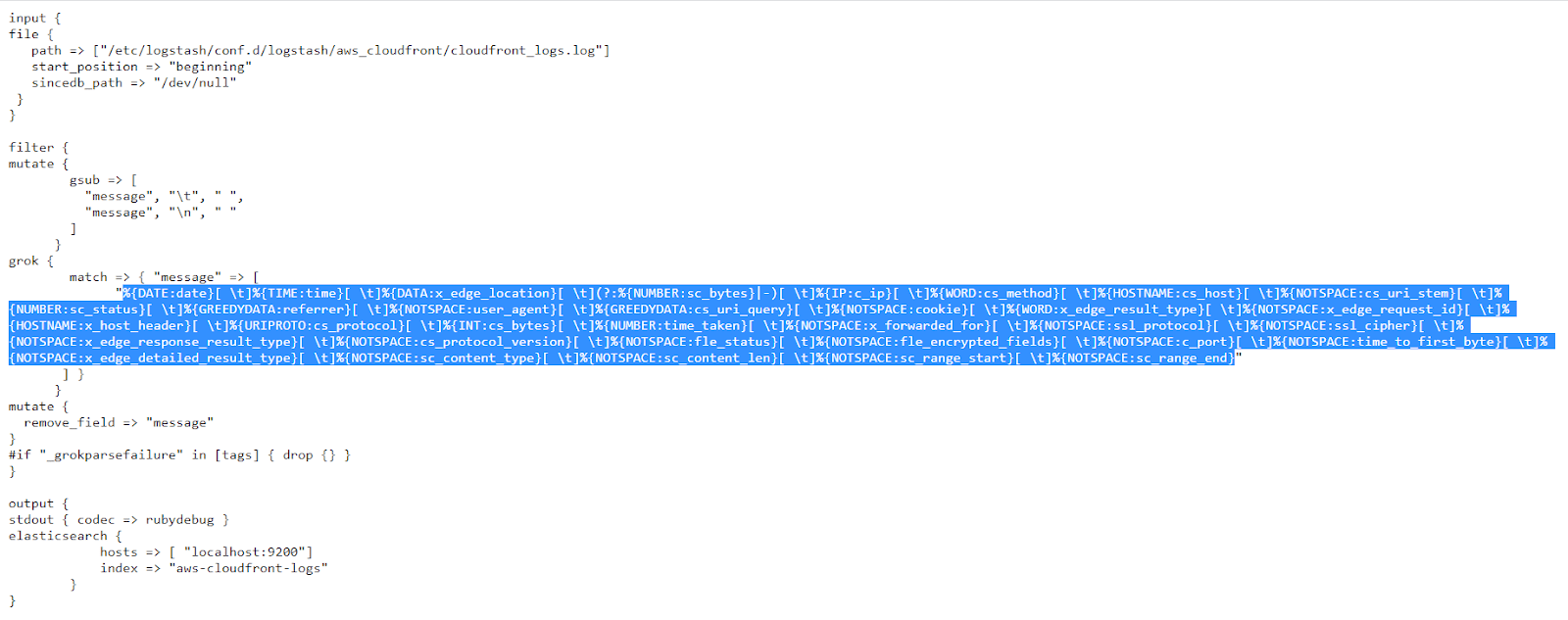
The configuration looks like this:

Original image link here

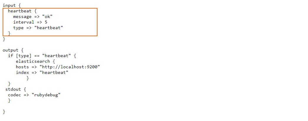
You can see there are two important settings in the “heartbeat” plugin namely the “message” and the “interval”. 

The “interval” value is in seconds and the heartbeat plugin will send the periodic messages in 5 seconds interval.

“message” setting will emit the specified string as the health indicator string. By default it will emit “ok”. We can give any value here. 

Let’s run logstash using the above configuration, by typing in the command:

sudo /usr/share/logstash/bin/logstash -f /etc/logstash/conf.d/logstash-input-plugins/heartbeat/heartbeat.conf

Wait for some time till the Logstash starts running and you can press CTRL+C after that. 

To view a sample document generated by the heartbeat plugin, you can type in the following request: 

curl -XGET "https://127.0.0.1:9200/heartbeat/_search?pretty=true" -H 'Content-Type: application/json' -d'{  "size": 1}'

This request will give the response as:

{
  "took" : 0,
  "timed_out" : false,
  "_shards" : {
    "total" : 1,
    "successful" : 1,
    "skipped" : 0,
    "failed" : 0
  },
  "hits" : {
    "total" : {
      "value" : 44,
      "relation" : "eq"
    },
    "max_score" : 1.0,
    "hits" : [
      {
        "_index" : "heartbeat",
        "_type" : "_doc",
        "_id" : "_ZOa-3IBngqXVfHU3YTf",
        "_score" : 1.0,
        "_source" : {
          "message" : "ok",
          "@timestamp" : "2020-06-28T15:45:29.966Z",
          "type" : "heartbeat",
          "host" : "es7",
          "@version" : "1"
        }
      }
    ]
  }
}

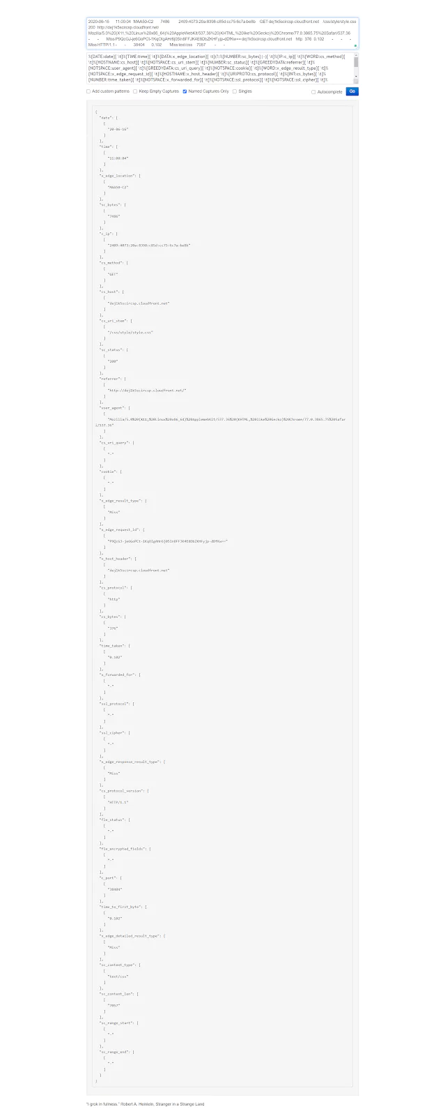
You can see the field named “message” with the specified string “ok” in the document. 

Now let’s explore other two different options that can be given to the “message” setting.

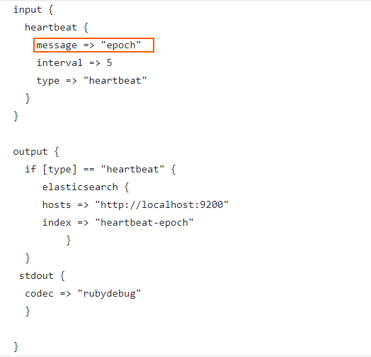
If we give the value “epoch” in the “message” setting, it will emit the time of the event as an epoch value under a field called “clock”.
Let’s replace the “ok” with the “epoch” for the “message” setting in our configuration. 

The updated configuration can be found in:

https://raw.githubusercontent.com/2arunpmohan/logstash-input-plugins/master/heartbeat/heartbeat-epoch.conf

The configuration would look like this

Original image link here

Let’s run Logstash with this configuration file using the command:

sudo /usr/share/logstash/bin/logstash -f /etc/logstash/conf.d/logstash-input-plugins/heartbeat/heartbeat-epoch.conf

Give some time for Logstash to run. After it has started running, wait for some time and then hit CTRL+C to quit the Logstash screen and to stop it.
Let’s inspect a single document from the index which we created now by typing in the request:

curl -XGET "https://127.0.0.1:9200/heartbeat-epoch/_search?pretty=true" -H 'Content-Type: application/json' -d'{  "size": 1}'

You can see that the document in the result looks like this:

{
        "_index" : "heartbeat-epoch",
        "_type" : "_doc",
        "_id" : "_ZOM_HIBngqXVfHUd6d_",
        "_score" : 1.0,
        "_source" : {
          "host" : "es7",
          "@timestamp" : "2020-06-28T20:09:23.480Z",
          "clock" : 1593374963,
          "type" : "heartbeat",
          "@version" : "1"
        }
      }

In this document, you can see that there is a field called “clock” which has the time in “epoch” representation. This is really helpful in scenarios where we need to calculate the delays in the ingestion pipelines using Logstash. The actual time of generation of an event and the time of ingestion can be subtracted to find the time delay in ingestion.  

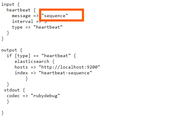
Also, the “message” setting can be set to have the value “sequence”, which basically will generate incrementing numbers in sequence under the field “clock”. The configuration of the logstash for this can be found in this link: 

https://raw.githubusercontent.com/2arunpmohan/logstash-input-plugins/master/heartbeat/heartbeat-sequence.conf

The configuration would look like this:

Original image link here 

Let’s run Logstash with this configuration file using the command:

sudo /usr/share/logstash/bin/logstash -f /etc/logstash/conf.d/logstash-input-plugins/heartbeat/heartbeat-sequence.conf

Give some time for Logstash to run. After it has started running, wait for some time and then hit CTRL+C to quit the Logstash screen and to stop it.

Let’s inspect a few documents from the index which we created now by typing in the request:

curl -XGET "https://127.0.0.1:9200/heartbeat-sequence/_search?pretty=true" -H 'Content-Type: application/json' -d'{ 
  "sort": [
    {
      "@timestamp": {
        "order": "asc"
      }
    }
  ]
}'

In the query, I have asked Elasticsearch to return the documents based on the ascending order of timestamps. 

You can see that the returned documents would look like below:

{
  "took" : 3,
  "timed_out" : false,
  "_shards" : {
    "total" : 1,
    "successful" : 1,
    "skipped" : 0,
    "failed" : 0
  },
  "hits" : {
    "total" : {
      "value" : 45,
      "relation" : "eq"
    },
    "max_score" : null,
    "hits" : [
      {
        "_index" : "heartbeat-sequence",
        "_type" : "_doc",
        "_id" : "5Db5FnMBfj_gbv8MHEss",
        "_score" : null,
        "_source" : {
          "@timestamp" : "2020-07-03T23:18:09.159Z",
          "clock" : 1
        },
        "sort" : [
          1593818289159
        ]
      },
      {
        "_index" : "heartbeat-sequence",
        "_type" : "_doc",
        "_id" : "5zb5FnMBfj_gbv8MKEuq",
        "_score" : null,
        "_source" : {
          "@timestamp" : "2020-07-03T23:18:14.023Z",
          "clock" : 2
        },
        "sort" : [
          1593818294023
        ]
      },
      {
        "_index" : "heartbeat-sequence",
        "_type" : "_doc",
        "_id" : "8Db5FnMBfj_gbv8MO0sn",
        "_score" : null,
        "_source" : {
          "@timestamp" : "2020-07-03T23:18:19.054Z",
          "clock" : 3
        },
        "sort" : [
          1593818299054
        ]
      },
      {
        "_index" : "heartbeat-sequence",
        "_type" : "_doc",
        "_id" : "Lzb5FnMBfj_gbv8MTkyz",
        "_score" : null,
        "_source" : {
          "@timestamp" : "2020-07-03T23:18:24.055Z",
          "clock" : 4
        },
        "sort" : [
          1593818304055
        ]
      },
      {
        "_index" : "heartbeat-sequence",
        "_type" : "_doc",
        "_id" : "NDb5FnMBfj_gbv8MYkwu",
        "_score" : null,
        "_source" : {
          "@timestamp" : "2020-07-03T23:18:29.056Z",
          "clock" : 5
        },
        "sort" : [
          1593818309056
        ]
      },
      {
        "_index" : "heartbeat-sequence",
        "_type" : "_doc",
        "_id" : "OTb5FnMBfj_gbv8MdUyz",
        "_score" : null,
        "_source" : {
          "@timestamp" : "2020-07-03T23:18:34.056Z",
          "clock" : 6
        },
        "sort" : [
          1593818314056
        ]
      },
      {
        "_index" : "heartbeat-sequence",
        "_type" : "_doc",
        "_id" : "PDb5FnMBfj_gbv8MiUxA",
        "_score" : null,
        "_source" : {
          "@timestamp" : "2020-07-03T23:18:39.056Z",
          "clock" : 7
        },
        "sort" : [
          1593818319056
        ]
      },
      {
        "_index" : "heartbeat-sequence",
        "_type" : "_doc",
        "_id" : "Qjb5FnMBfj_gbv8MnEzH",
        "_score" : null,
        "_source" : {
          "@timestamp" : "2020-07-03T23:18:44.057Z",
          "clock" : 8
        },
        "sort" : [
          1593818324057
        ]
      },
      {
        "_index" : "heartbeat-sequence",
        "_type" : "_doc",
        "_id" : "RDb5FnMBfj_gbv8MsExQ",
        "_score" : null,
        "_source" : {
          "@timestamp" : "2020-07-03T23:18:49.057Z",
          "clock" : 9
        },
        "sort" : [
          1593818329057
        ]
      },
      {
        "_index" : "heartbeat-sequence",
        "_type" : "_doc",
        "_id" : "Rzb5FnMBfj_gbv8MxEwD",
        "_score" : null,
        "_source" : {
          "@timestamp" : "2020-07-03T23:18:54.057Z",
          "clock" : 10
        },
        "sort" : [
          1593818334057
        ]
      }
    ]
  }
}

Here the field “clock” can be seen with incrementing numbers and has been sent in every 5 seconds. This is also helpful in determining missed events.

Generate Input plugin

Sometimes for testing or other purposes it would be great to have some specified data to be inserted. The conditions might vary like you might want to have some specific data generated for longer times, or some data generated for some iterations etc. Of course we can write custom scripts or programs to generate such data and send to a file or even Logstash directly. But there is a much more simple way to do such things within Logstash itself. We can use the generator plugin for logstash to generate random/custom log events. 

Let’s dive into an example first. 

The configuration for the example can be seen in the link

https://raw.githubusercontent.com/2arunpmohan/logstash-input-plugins/master/generator/generator.conf

The configuration would look like this:

Original image link here

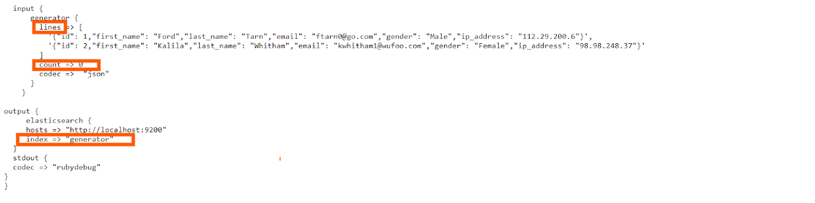
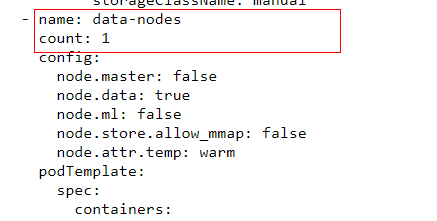
In the configuration, under the “lines” section, two JSON documents were given and also for the Logstash to understand it is JSON, we have specified the “codec” value as JSON.
Now, “count” parameter is set to 0, which basically tells the Logstash to generate an infinite number of events with the values in the “lines” array.
If we set any other number for the “count” parameter, Logstash will generate each line that many times. 

Let’s run Logstash with this configuration file using the command:

sudo /usr/share/logstash/bin/logstash -f /etc/logstash/conf.d/logstash-input-plugins/generator/generator.conf

Give some time for Logstash to run. After it has started running, wait for some time and then hit CTRL+C to quit the Logstash screen and to stop it.

Let’s inspect a single document from the index which we created now by typing in the request:

curl -XGET "https://127.0.0.1:9200/generator/_search?pretty=true" -H 'Content-Type: application/json' -d'{  "size": 1}'

You can see that the document in the result looks like this:

{
        "_index" : "generator",
        "_type" : "_doc",
        "_id" : "oDYqF3MBfj_gbv8MqlUB",
        "_score" : 1.0,
        "_source" : {
          "last_name" : "Tarn",
          "sequence" : 0,
          "gender" : "Male",
          "host" : "es7",
          "@version" : "1",
          "@timestamp" : "2020-07-04T00:12:16.363Z",
          "email" : "ftarn0@go.com",
          "id" : 1,
          "ip_address" : "112.29.200.6",
          "first_name" : "Ford"
        }
}

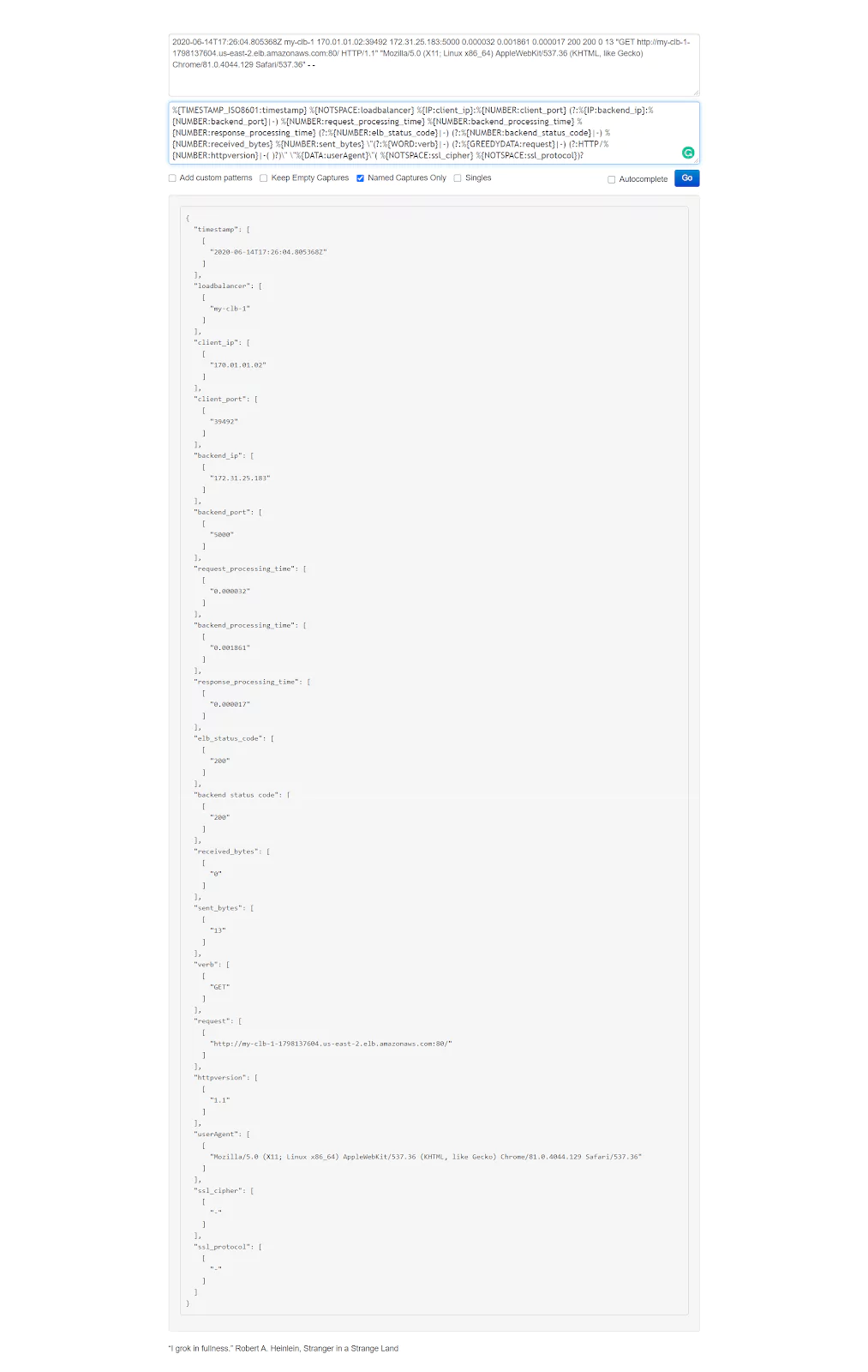
This plugin is very useful when we need to have documents generated for testing. We can give multiple lines and test grok patterns or filters and see how they are getting indexed using this plugin.

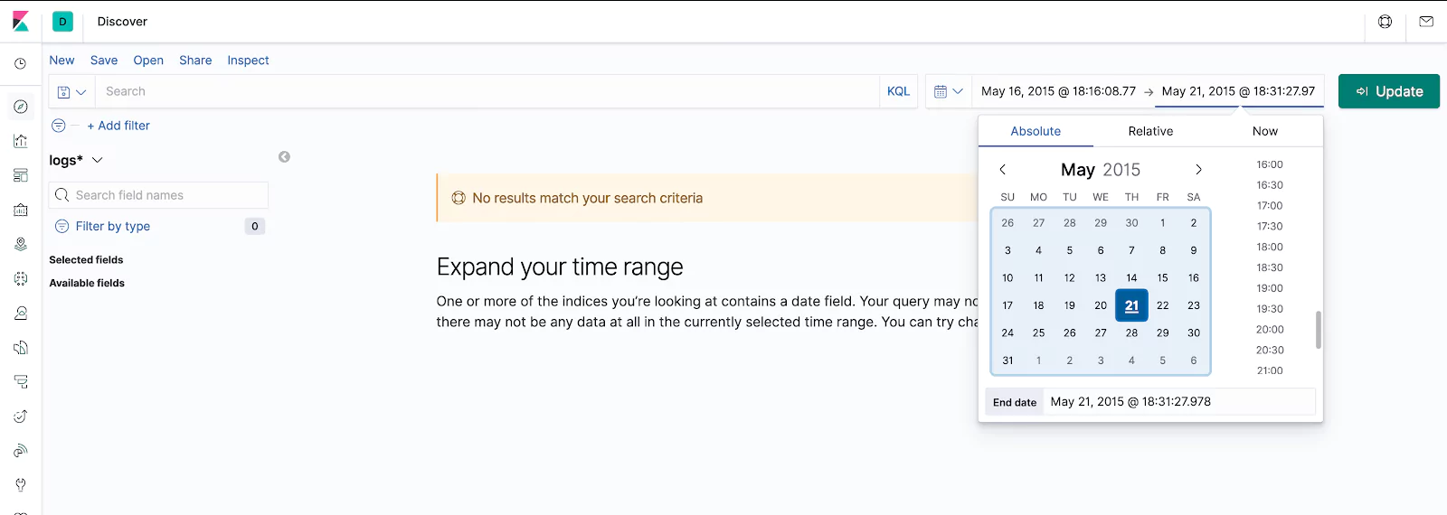
Dead letter queue

This is one important input plugin and is an immensely helpful one too. So far we have seen the cases of successful processing of events by Logstash. Now what happens when Logstash fails to process an event? Normally the event is dropped and hence we will lose it. 

In many cases it would be helpful to collect those documents for further inspection and do the necessary actions so that in future the event dropping won’t happen. 

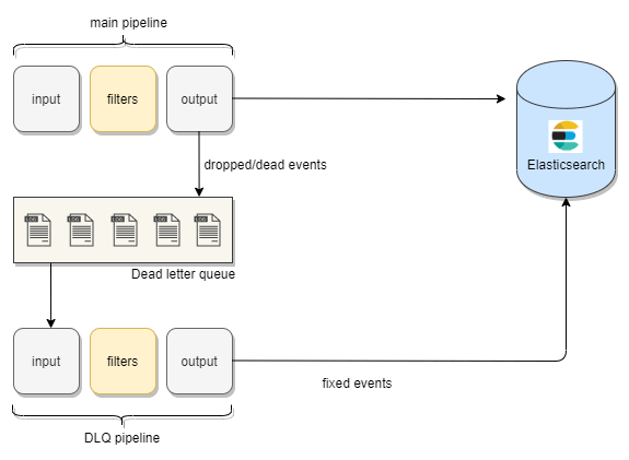
To make this possible Logstash provides us with a queue called dead-letter-queue. The events which are dropped would get collected here. 

Now, once in the dead-letter-queue, with the help of this dead-letter-queue input plugin , we can process these documents using another Logstash configuration and make the necessary changes and then index them back to Elasticsearch.

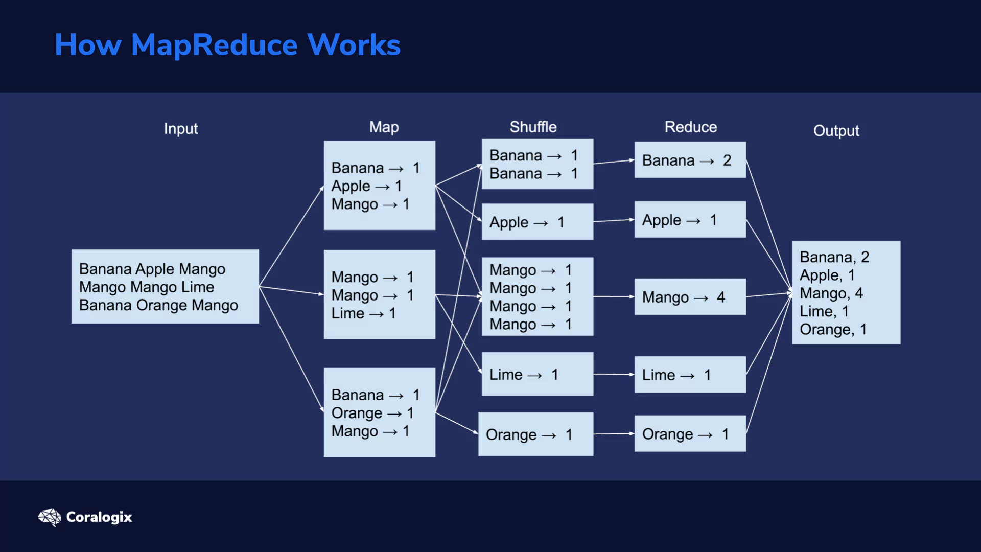
 You can see the flow of unprocessed events to dead-letter-queue and then to Elasticsearch in this diagram.

Original image link here 

So that we have seen what is “dead-letter-queue” in Logstash, let’s move on to a simple use case involving the dead letter queue input plugin. 

Since we are using the dead-letter-queue input plugin, we need to do two things prior.
First, we need to enable the dead-letter-queue.

Second, we need to set the path to the dead-letter-queue. 

Let’s create a folder named dlq to store the dead-letter-queue data by typing in the following command

mkdir /home/student/dlq

Now, Logstash creates a user named “logstash” during the installation and performs the actions using this user. So let’s change the ownership of the above folder to the user named “logstash” by typing in the following command

sudo chown -R logstash:logstash /home/student/dlq

Now let’s enable the dead_letter_queue and also specify its path in the logstash’s setting by editing the settings file by typing in

sudo nano /etc/logstash/logstash.yml

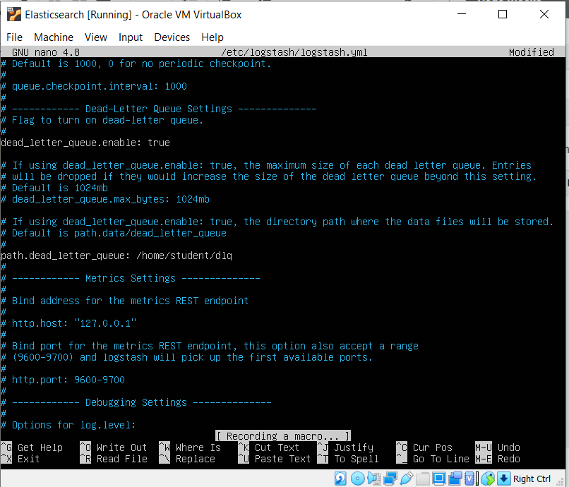
Now uncomment the setting dead_letter_queue and give the value as true  

Also give set the path to store the queue data, by uncommenting the path.dead_letter_queue as /home/student/dlq    

The sections of the logstash.yml file will look like this after we have made the necessary edits

Original image link here 

To save our file, we press CTRL+X, then press Y, and finally ENTER.

Now let’s input a few documents from a JSON file. 

Let’s have a look at the documents in the file by opening the file using the command

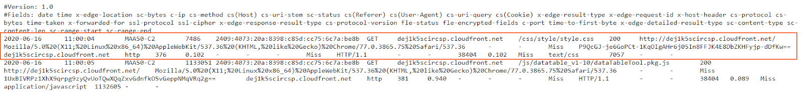
cat /etc/logstash/conf.d/logstash-input-plugins/sample-data.json

Original image link here

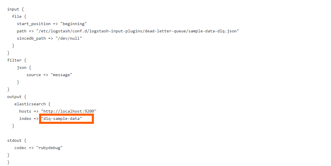
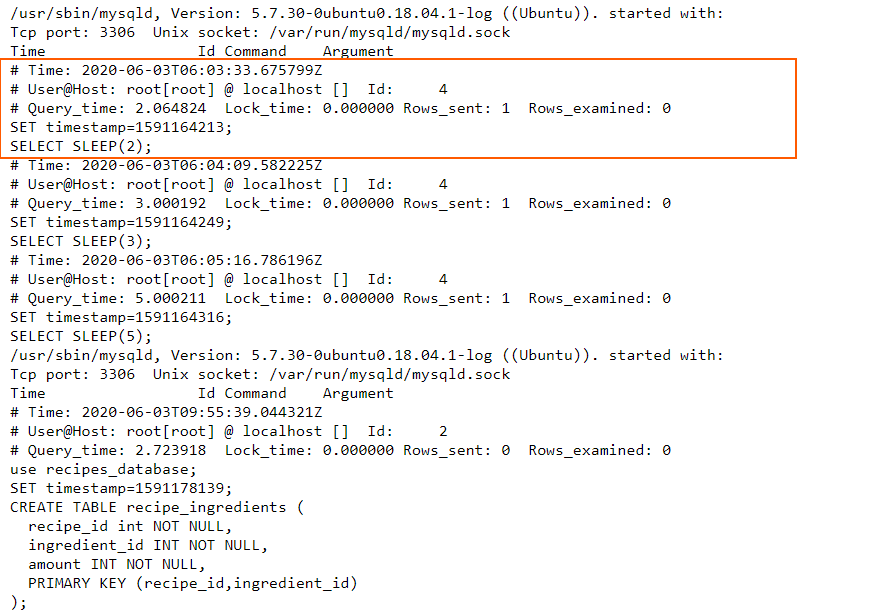
You can see that, in the first 10 documents, the “age” field has integer values. But from the 11th document, it is mistakenly given as boolean. So what happens is that Elasticsearch will assign a type “long” data type used for the integers for the “age” field. This is because, when we are indexing the documents the first document which has the “age” as integers are indexed first, so Elasticsearch will assign them the “age” field. Now, when the 11th document comes with the boolean value for “age” , Elasticsearch will reject the document since a field cannot contain two data types. So it does for all the documents with “age” as a boolean value.

So let’s index the sample data and see what happens. 

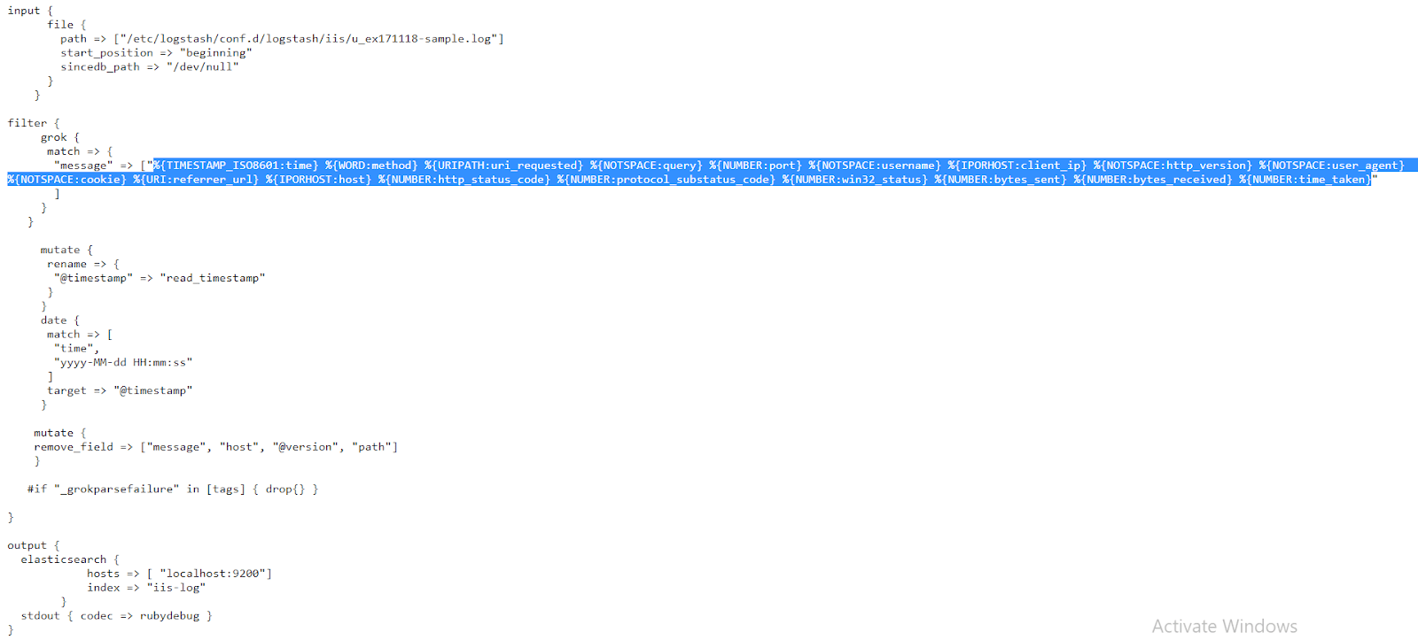
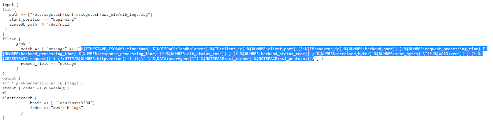
For that let’s run the configuration file for logstash. Let’s have a look at the configuration file by going to the following link:

https://raw.githubusercontent.com/2arunpmohan/logstash-input-plugins/master/dead-letter-queue/dlq-data-01-ingest.conf

The configuration file would look like this:

You can type in this command to run Logstash for indexing the sample data 

sudo /usr/share/logstash/bin/logstash --path.settings /etc/logstash -f /etc/logstash/conf.d/dead-letter-queue/dlq-data-01.conf

In the command we typed, there is an extra parameter called “path.settings” and its value “/etc/logstash”. This is given so that Logstash will understand where the logstash.yml file is located and will take that settings.

Give some time for Logstash to run. After it has started running, wait for some time and then hit CTRL+C to quit the Logstash screen and to stop it.

Let’s inspect how many documents were inserted to the index. There was a total of 20 documents and out of it only 10 should have been indexed as the other 10 would have the mapping issue. 

curl -XGET "https://127.0.0.1:9200/dlq-sample-data/_search?pretty=true" -H 'Content-Type: application/json' -d'{  "track_total_hits": true, size:0}'

You can see that the response will looks like this:

{
  "took" : 0,
  "timed_out" : false,
  "_shards" : {
    "total" : 1,
    "successful" : 1,
    "skipped" : 0,
    "failed" : 0
  },
  "hits" : {
    "total" : {
      "value" : 10,
      "relation" : "eq"
    },
    "max_score" : 1.0,
    "hits" : [
      {
        "_index" : "dlq-sample-data",
        "_type" : "_doc",
        "_id" : "G2v1GHMBfj_gbv8MTzae",
        "_score" : 1.0,
        "_source" : {
          "@timestamp" : "2020-07-04T08:33:14.322Z",
          "@version" : "1",
          "gender" : "Female",
          "host" : "es7",
          "message" : """{"age":39,"full_name":"Shelley Bangs","gender":"Female"}""",
          "path" : "/etc/logstash/conf.d/logstash-input-plugins/dead-letter-queue/sample-data-dlq.json",
          "age" : 39,
          "full_name" : "Shelley Bangs"
        }
      }
    ]
  }
}

In the response you can see that the hits.total.value is equal to 10 (marked in bold in the above response). 

Now you can see that the remaining 10 documents are not indexed.So these documents are dropped and since we have enabled the dead_letter_queue, these documents should be there.
Let’s use the input plugin for reading from the dead_letter_queue. 

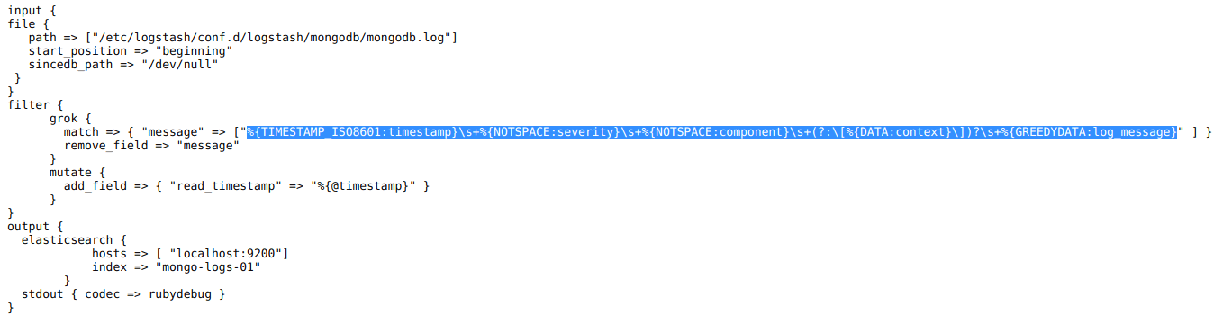
The configuration for reading from the dead_letter_queue can be seen in this link:

https://raw.githubusercontent.com/2arunpmohan/logstash-input-plugins/master/dead-letter-queue/dlq.conf

The configuration looks like this

Original image link here 

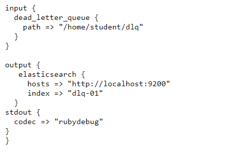
In the configuration, we have pointed to the path where we had set the dead_letter_queue. Now if we run the configuration Logstash will read the contents in the dead_letter_queue and process it and then index to Elasticsearch. 

For the sake of simplicity , in the configuration, I have not added any filters. We definitely can add filters depending up on the use case and then run the configuration if we want. 

Let’s run Logstash with this configuration file using the command:

sudo /usr/share/logstash/bin/logstash --path.settings /etc/logstash -f /etc/logstash/conf.d/logstash-input-plugins/dead-letter-queue/dlq.conf

Give some time for Logstash to run. After it has started running, wait for some time and then hit CTRL+C to quit the Logstash screen and to stop it.

Let’s inspect the number of documents that were indexed now by typing in the request:

curl -XGET "https://127.0.0.1:9200/dlq-01/_search?pretty=true" -H 'Content-Type: application/json' -d'{  "size": 1}'

The response to the request will return this.

{
  "took" : 0,
  "timed_out" : false,
  "_shards" : {
    "total" : 1,
    "successful" : 1,
    "skipped" : 0,
    "failed" : 0
  },
  "hits" : {
    "total" : {
      "value" : 10,
      "relation" : "eq"
    },
    "max_score" : 1.0,
    "hits" : [
      {
        "_index" : "dlq-01",
        "_type" : "_doc",
        "_id" : "O2thGnMBfj_gbv8MJmR4",
        "_score" : 1.0,
        "_source" : {
          "@timestamp" : "2020-07-04T08:33:14.502Z",
          "full_name" : "Robbyn Narrie",
          "gender" : "Female",
          "@version" : "1",
          "path" : "/etc/logstash/conf.d/logstash-input-plugins/dead-letter-queue/sample-data-dlq.json",
          "host" : "es7",
          "message" : """{"age":false,"full_name":"Robbyn Narrie","gender":"Female"}""",
          "age" : false
        }
      }
    ]
  }
}

You can see that there are 10 documents that were indexed. And upon inspection on the sample document, it has returned the document which had the boolean value for the field “age”. 

Note that with this configuration, after running the Logstash, the queue contents would not be cleared. If you want the documents which were read not to be indexed again, the flag “commit_offsets” to true, just under the “path” setting.

Http_poller plugin

The http_poller plugin is a very useful input plugin that comes with Logstash. As the name indicates, this plugin can be used to poll http endpoints periodically and let us store the response in Elasticsearch. 

This can be helpful if we have health APIs exposed for our applications and need periodic status monitoring of them. Also we can use it to collect the status like weather, match details etc periodically. 

In our case let’s look at polling two http APIs for the purpose of understanding the plugin. We will first call a POST method to an external API at an interval of 5 seconds, and will store it to an index named “http-poller-api”. Then we will also call the Elasticsearch’s cluster health API, which is a GET request , in every second and store it in an index named “http-poller-es-health”. 

Let’s first familiarize with both of the APIs first. 

The first API is a simple online free API, which gives some response when we give a POST request. 

Open the website apitester.com and a web page will open like this. We open this website simply to test one of the APIs we are trying to call.

Original image link here 

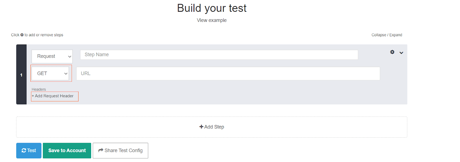
Now change the value GET to POST from the dropdown and also click on the “Add Request Header”. The resulting window would look like this:

Original image link here

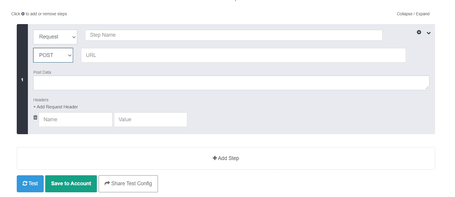
Now, fill the box marked as URL with this address https://jsonplaceholder.typicode.com/posts
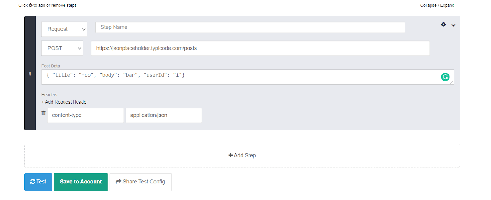
In the section post data, add the following JSON lines

{ "title": "foo", "body": "bar", "userId": "1"}

And add  “content-type” and “application/json” as the key value pairs for the boxes named “name” and “value” respectively.
The filled form details would look like this: 

Original image link here 

Now press the “Test” button and you can see the response details as below:

Original image link here

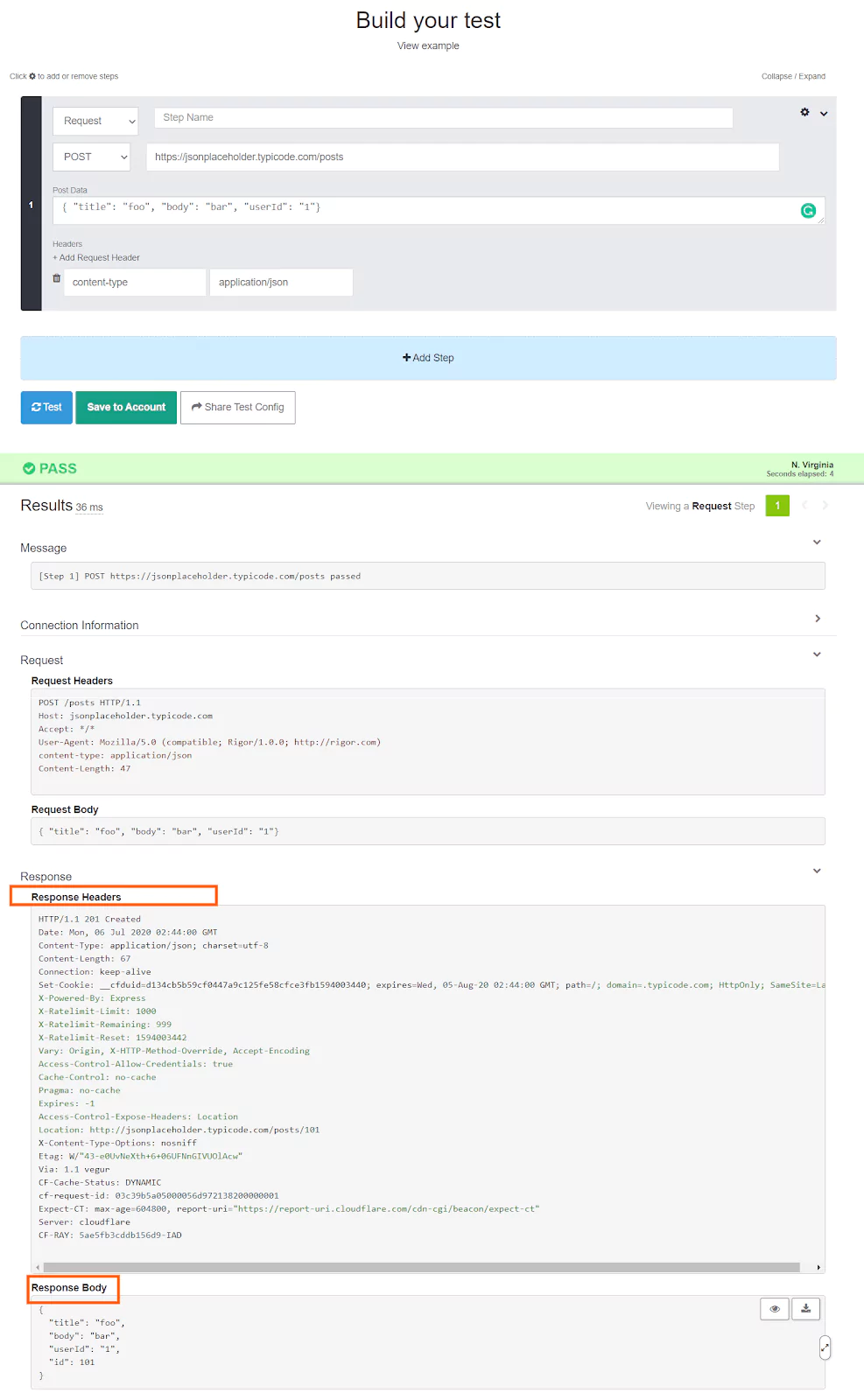
What this API does is that it will create a record in the remote database and send the details with the record id as the response body. You can also see a pretty long response header also along with the response. 

Our second API is a GET request supplied by our own Elasticsearch itself, which gives us the cluster status. You can test the API by typing in the following request in the terminal 

curl -XGET "https://localhost:9200/_cluster/health"

This will result in the following response:

{
  "cluster_name" : "elasticsearch",
  "status" : "yellow",
  "timed_out" : false,
  "number_of_nodes" : 1,
  "number_of_data_nodes" : 1,
  "active_primary_shards" : 56,
  "active_shards" : 56,
  "relocating_shards" : 0,
  "initializing_shards" : 0,
  "unassigned_shards" : 50,
  "delayed_unassigned_shards" : 0,
  "number_of_pending_tasks" : 0,
  "number_of_in_flight_fetch" : 0,
  "task_max_waiting_in_queue_millis" : 0,
  "active_shards_percent_as_number" : 52.83018867924528
}

Now that we have familiarised both the API calls , let’s have a look at the configuration for logstash. You can see the configuration in this link:

https://raw.githubusercontent.com/2arunpmohan/logstash-input-plugins/master/http-poller/http-poller.conf

The configuration would look like this:

Original image link here

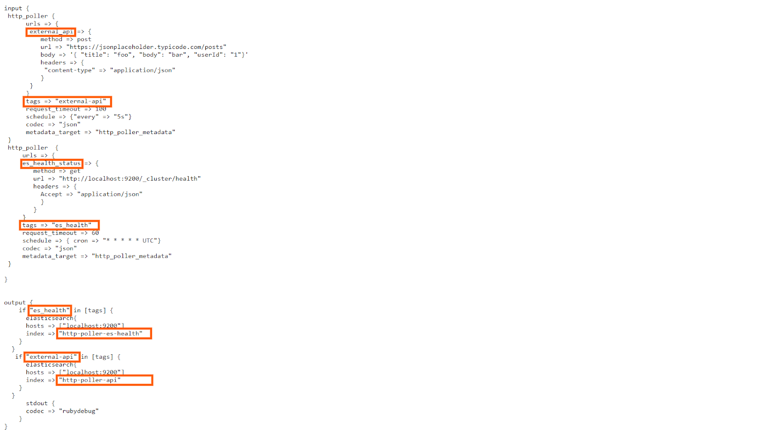
In the configuration you can see two “http_poller” sections. One is named as “external_api” and the other is named as “es_health_status”.
In the “external_api” section , you can see the URL we have called in the first example, with the method, and the content-type mentioned in the “headers” section.
Apart from that, I have given an identifier named “external-api” in the “tags” to identify the response from this section. 

Also the periodic scheduling is done every 5 seconds. This is specified under the “schedule” section.
Another important setting is the “metadata_target”. I have specified that to be “http_poller_metadata”. This will ensure that the response headers will be stored in the field named “http_poller_metadata” when storing in ES. 

Similar settings are applied to the “es_health_status” section too. Here the difference is that the “method” is a GET method and also the “Schedule” section is given a cron expression as the value. Also the value of “tags” is “es_health”. 

Now coming to the output section, there is a check on the “tags” field. If the data is coming from the “external-api” tag, the index where the data is stored is “http-poller-api”. But if the data contains “tags” value as “es_health”, it will be stored in the index named “http-poller-es-health”. 

Since we have a good understanding of the Logstash configuration, let’s run this configuration by typing in this command

sudo /usr/share/logstash/bin/logstash -f /etc/logstash/conf.d/logstash-input-plugins/http_poller/http_poller.conf

Wait for some time for the logstash to run. Since it is a polling operation, Logstash won’t finish running,but will keep running. So after about 5 mins, you can stop the Logstash by hitting CTRL+C 

Now let’s check whether we have data in both of the indices. Lets first query the index “http-poller-api” with this query:

curl -XGET "https://localhost:9200/http-poller-api/_search?pretty=true" -H 'Content-Type: application/json' -d'{
  "query": {
    "match_all": {
    }
  },
  "size": 1,
  "sort": [
    {
      "@timestamp": {
        "order": "desc"
      }
    }
  ]
}'

This will return a single document like this:

{
  "took" : 2,
  "timed_out" : false,
  "_shards" : {
    "total" : 1,
    "successful" : 1,
    "skipped" : 0,
    "failed" : 0
  },
  "hits" : {
    "total" : {
      "value" : 463,
      "relation" : "eq"
    },
    "max_score" : null,
    "hits" : [
      {
        "_index" : "http-poller-api",
        "_type" : "_doc",
        "_id" : "YGw8InMBfj_gbv8MmFqD",
        "_score" : null,
        "_source" : {
          "userId" : "1",
          "id" : 101,
          "@timestamp" : "2020-07-06T03:47:43.258Z",
          "http_poller_metadata" : {
            "request" : {
              "headers" : {
                "content-type" : "application/json"
              },
              "body" : """{ "title": "foo", "body": "bar", "userId": "1"}""",
              "method" : "post",
              "url" : "https://jsonplaceholder.typicode.com/posts"
            },
            "response_headers" : {
              "server" : "cloudflare",
              "expires" : "-1",
              "x-ratelimit-limit" : "1000",
              "content-length" : "67",
              "access-control-expose-headers" : "Location",
              "access-control-allow-credentials" : "true",
              "x-content-type-options" : "nosniff",
              "via" : "1.1 vegur",
              "pragma" : "no-cache",
              "etag" : "W/"43-e0UvNeXth+6+06UFNnGIVUOlAcw"",
              "date" : "Mon, 06 Jul 2020 03:47:43 GMT",
              "location" : "https://jsonplaceholder.typicode.com/posts/101",
              "cf-ray" : "5ae6588feab20000-SIN",
              "cache-control" : "no-cache",
              "connection" : "keep-alive",
              "content-type" : "application/json; charset=utf-8",
              "x-powered-by" : "Express",
              "x-ratelimit-reset" : "1594007283",
              "cf-cache-status" : "DYNAMIC",
              "expect-ct" : "max-age=604800, report-uri="https://report-uri.cloudflare.com/cdn-cgi/beacon/expect-ct"",
              "vary" : "Origin, X-HTTP-Method-Override, Accept-Encoding",
              "x-ratelimit-remaining" : "991",
              "cf-request-id" : "03c3d5adf3000100d3bf307200000001"
            },
            "code" : 201,
            "name" : "external_api",
            "response_message" : "Created",
            "times_retried" : 0,
            "runtime_seconds" : 0.576409,
            "host" : "es7"
          },
          "@version" : "1",
          "body" : "bar",
          "title" : "foo",
          "tags" : [
            "external-api"
          ]
        },
        "sort" : [
          1594007263258
        ]
      }
    ]
  }
}

In the response, you can see the “http_poller_metadata” field with the necessary details of both the request and response headers. Also there is the field named “id” returned by the server. 

Now coming to the index “http-poller-es-health”, lets query the same query like this:

curl -XGET "https://localhost:9200/http-poller-es-health/_search?pretty=true" -H 'Content-Type: application/json' -d'{
  "query": {
    "match_all": {
      
    }
  },
  "size": 1,
  "sort": [
    {
      "@timestamp": {
        "order": "desc"
      }
    }
  ]
}'

This will return document like this:

{
  "took" : 0,
  "timed_out" : false,
  "_shards" : {
    "total" : 1,
    "successful" : 1,
    "skipped" : 0,
    "failed" : 0
  },
  "hits" : {
    "total" : {
      "value" : 39,
      "relation" : "eq"
    },
    "max_score" : null,
    "hits" : [
      {
        "_index" : "http-poller-es-health",
        "_type" : "_doc",
        "_id" : "PWw7InMBfj_gbv8M8Fqg",
        "_score" : null,
        "_source" : {
          "number_of_pending_tasks" : 0,
          "task_max_waiting_in_queue_millis" : 0,
          "active_shards_percent_as_number" : 52.83018867924528,
          "status" : "yellow",
          "relocating_shards" : 0,
          "initializing_shards" : 0,
          "unassigned_shards" : 50,
          "active_primary_shards" : 56,
          "active_shards" : 56,
          "delayed_unassigned_shards" : 0,
          "timed_out" : false,
          "@version" : "1",
          "tags" : [
            "es_health"
          ],
          "cluster_name" : "elasticsearch",
          "@timestamp" : "2020-07-06T03:47:00.279Z",
          "number_of_in_flight_fetch" : 0,
          "number_of_nodes" : 1,
          "http_poller_metadata" : {
            "request" : {
              "headers" : {
                "Accept" : "application/json"
              },
              "method" : "get",
              "url" : "https://localhost:9200/_cluster/health"
            },
            "response_headers" : {
              "content-type" : "application/json; charset=UTF-8"
            },
            "code" : 200,
            "name" : "es_health_status",
            "response_message" : "OK",
            "times_retried" : 0,
            "runtime_seconds" : 0.0057480000000000005,
            "host" : "es7"
          },
          "number_of_data_nodes" : 1
        },
        "sort" : [
          1594007220279
        ]
      }
    ]
  }
}

Here also you can see the same.
So by using this input plugin we can call HTTP calls periodically index the response with necessary data to a single index or multiple indices. 

Twitter plugin

Another interesting input plugin which is provided by Logstash is the Twitter plugin. Twitter input plugin allows us to stream Twitter events directly to Elasticsearch or any output that Logstash support. 

Let’s explore the Twitter input plugin and see it in action. 

For this to work, you need to have a Twitter account. If you don’t have one, don’t worry, just go to Twitter and create one using the signup option. 

Now once you have your Twitter account, go to
https://developer.twitter.com/en/apps 

This is the developer portal of Twitter. You can see the screen like this

Original image link here 

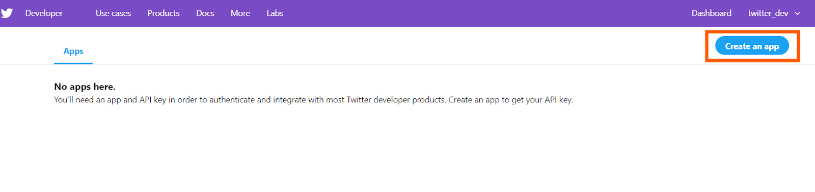
Click on the “create an app” button. If you are creating an app for the first time, it would ask to “apply” and it might take a day or two to get the approval. So once you have the approval, the “create an app” clicking would redirect to a screen like this:

Original image link here

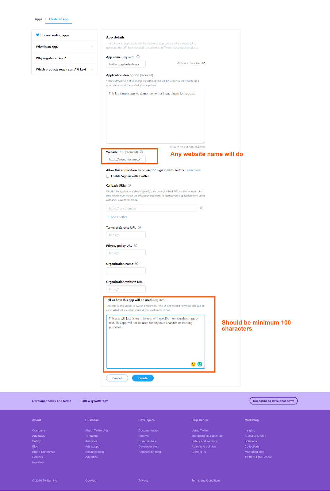
After pressing the “create” button in the bottom, it will ask once again for confirmation with the updated terms and conditions like this:

Original image link here 

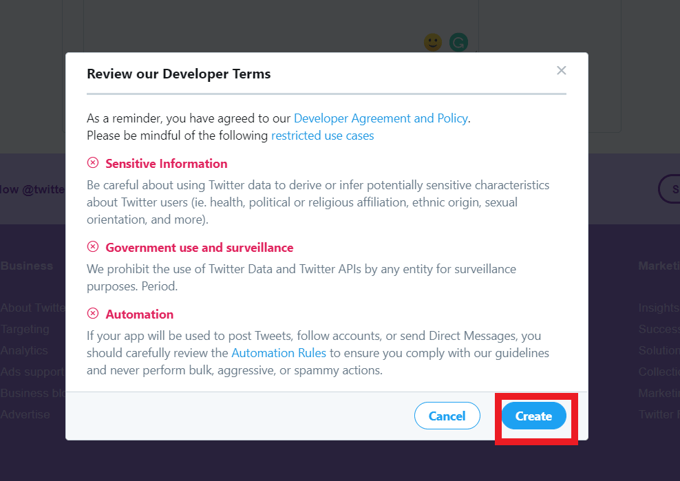
Clicking on the “create” button will create the app for us and you will see the screen like this

Original image link here 

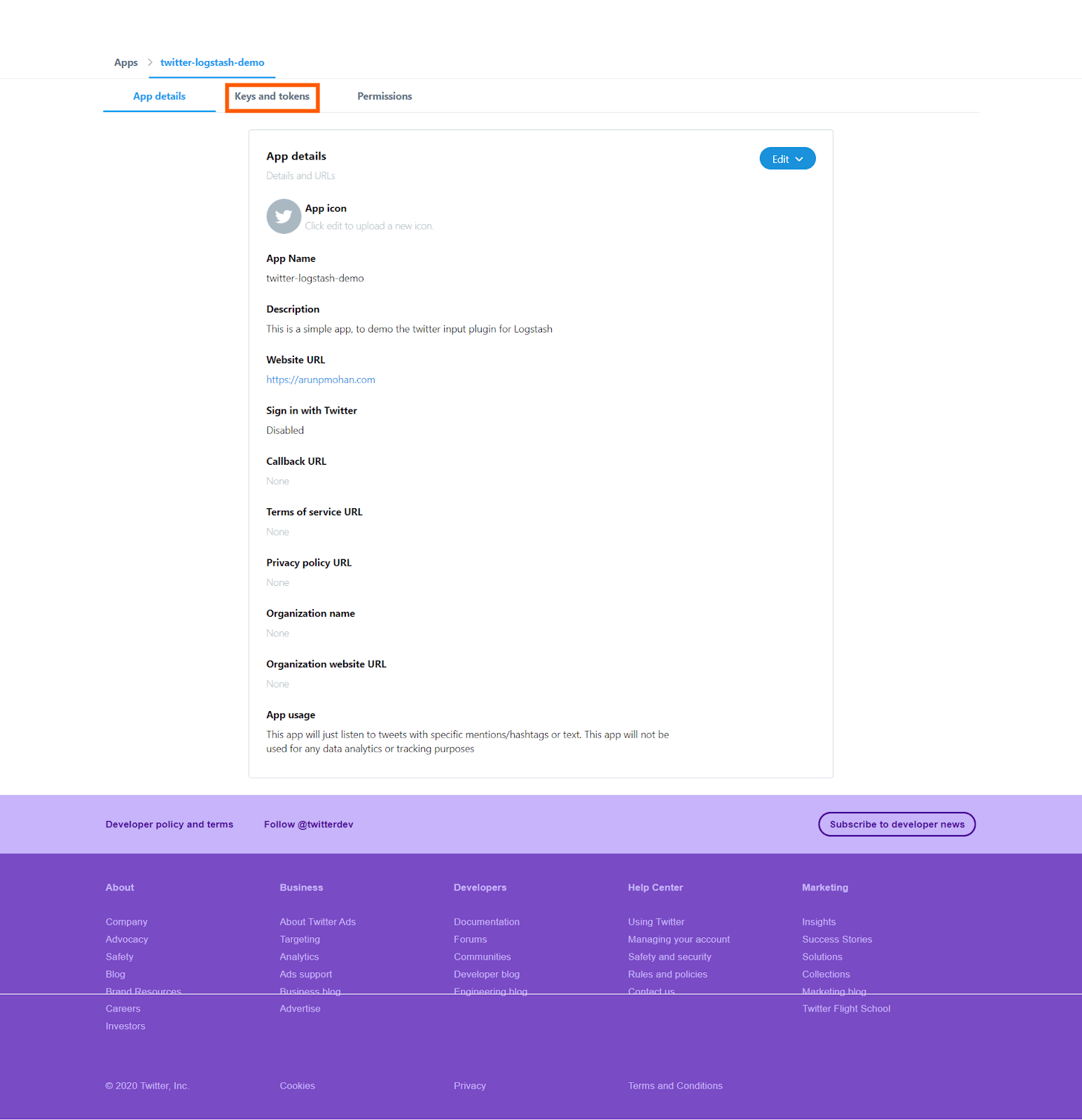
In the screen you can see three tabs, press the “keys and tokens” tab and you will see this screen, which contains the necessary keys and tokens

Original image link here

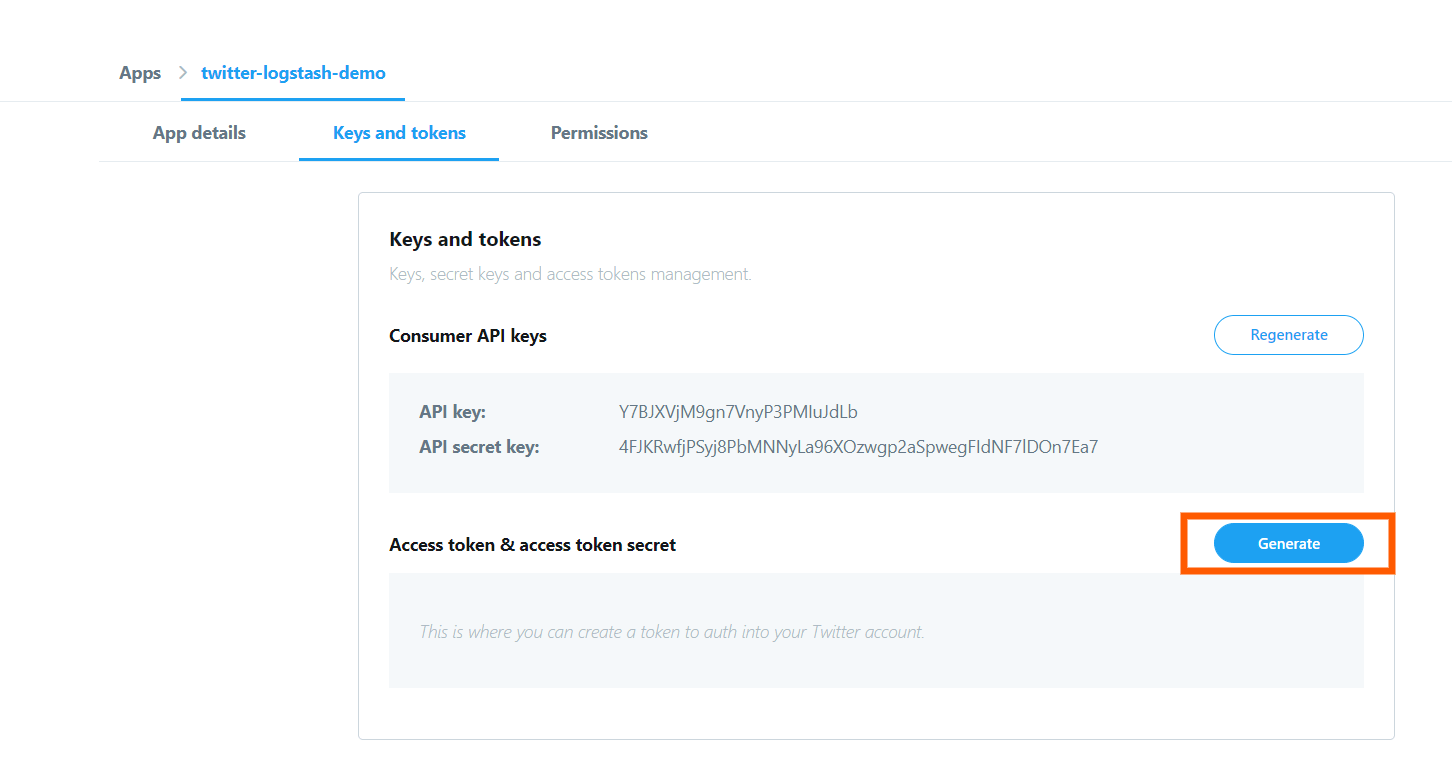
From this screen copy the “api key” and “api secret key” values to a notepad or so.

In the screen, press the “generate” button and the “access token” and “access token secret” will be generated for you like this:

Original image link here

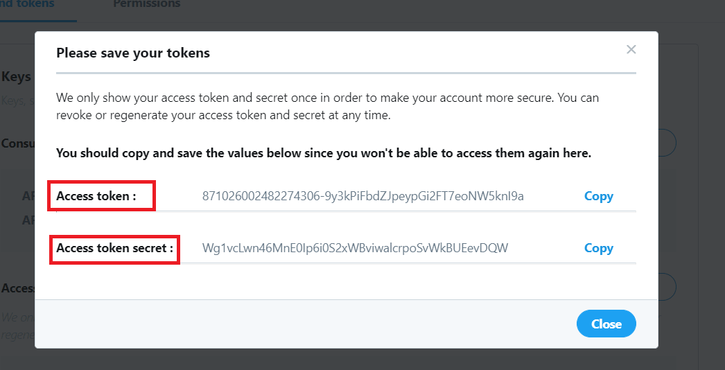
Now copy this information and keep them along with the “api key” and “api secret key” which you copied earlier in the notepad.

Now the information collected in the notepad will have the following details

Original image link here 

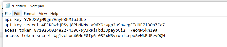
Now we have the necessary information to proceed to use the Twitter plugin for Logstash. 

Let’s look directly at the configuration file of this setup in this link:

https://raw.githubusercontent.com/2arunpmohan/logstash-input-plugins/master/twitter/twitter.conf

The configuration would look like this

original image link here 

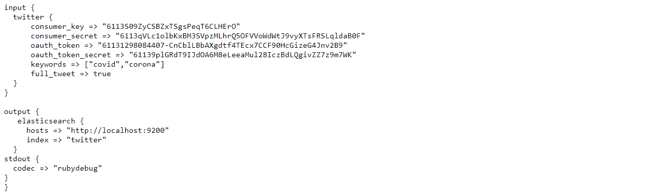
Now enter the value of

“api key” which we copied to the notepad to that of the “consumer_key”

“api key secret” to that of the “consumer_secret”

“Access token” to that of the “oauth_token”

“Access token secret” to that of the “oauth_token_secret” 

You can enter any string values in the “keywords” section which will get you the tweets which contains those strings. Here I have given “covid”, “corona” as the strings. This will give tweets which contain either “covid” OR “corona” in their body. 

The “full_tweet” value is set to true to get the full information about the tweet as given by the Twitter

Let’s run Logstash with this configuration file using the command:

sudo /usr/share/logstash/bin/logstash -f /etc/logstash/conf.d/logstash-input-plugins/twitter/twitter.conf

Give some time for Logstash to run. After it has started running, wait for some time and then hit CTRL+C to quit the Logstash screen and to stop it.

Let’s inspect a single document from the index which we created now by typing in the request:

curl -XGET "https://127.0.0.1:9200/twitter/_search?pretty=true" -H 'Content-Type: application/json' -d'{  "size": 1}'

You can see that the document in the result looks like this:

{
  "took" : 0,
  "timed_out" : false,
  "_shards" : {
    "total" : 1,
    "successful" : 1,
    "skipped" : 0,
    "failed" : 0
  },
  "hits" : {
    "total" : {
      "value" : 115,
      "relation" : "eq"
    },
    "max_score" : 1.0,
    "hits" : [
      {
        "_index" : "twitter",
        "_type" : "_doc",
        "_id" : "OZNS-XIBngqXVfHUK0_d",
        "_score" : 1.0,
        "_source" : {
          "quote_count" : 0,
          "reply_count" : 0,
          "lang" : "en",
          "@version" : "1",
          "retweeted" : false,
          "coordinates" : null,
          "text" : "RT @beatbyanalisa: My biggest fear about contracting COVID is not getting sick, it's me unknowingly passing it along to someone else... And...",
          "in_reply_to_screen_name" : null,
          "is_quote_status" : false,
          "geo" : null,
          "favorite_count" : 0,
          "favorited" : false,
          "created_at" : "Sun Jun 28 05:06:43 +0000 2020",
          "retweeted_status" : {
            "quote_count" : 6,
            "reply_count" : 8,
            "lang" : "en",
            "retweeted" : false,
            "coordinates" : null,
            "text" : "My biggest fear about contracting COVID is not getting sick, it's me unknowingly passing it along to someone else..... https://t.co/Hh3mMNUewS",
            "in_reply_to_screen_name" : null,
            "is_quote_status" : false,
            "geo" : null,
            "extended_tweet" : {
              "full_text" : "My biggest fear about contracting COVID is not getting sick, it's me unknowingly passing it along to someone else... And then that someone may not be able to handle it as well as I may be able to. That's what scares me the most.",
              "display_text_range" : [
                0,
                228
              ],
              "entities" : {
                "hashtags" : [ ],
                "symbols" : [ ],
                "user_mentions" : [ ],
                "urls" : [ ]
              }
            },
            "favorite_count" : 87,
            "favorited" : false,
            "created_at" : "Sun Jun 28 01:06:16 +0000 2020",
            "truncated" : true,
            "retweet_count" : 46,
            "in_reply_to_status_id_str" : null,
            "in_reply_to_user_id" : null,
            "place" : null,
            "id" : 1277045619723558914,
            "filter_level" : "low",
            "user" : {
              "followers_count" : 1386,
              "friends_count" : 1032,
              "translator_type" : "none",
              "profile_background_color" : "000000",
              "profile_image_url" : "https://pbs.twimg.com/profile_images/1247544253015867394/wNFFsE6l_normal.jpg",
              "default_profile" : false,
              "lang" : null,
              "profile_background_image_url" : "https://abs.twimg.com/images/themes/theme9/bg.gif",
              "screen_name" : "beatbyanalisa",
              "profile_background_image_url_https" : "https://abs.twimg.com/images/themes/theme9/bg.gif",
              "geo_enabled" : true,
              "utc_offset" : null,
              "name" : """""",
              "listed_count" : 24,
              "profile_link_color" : "F76BB5",
              "statuses_count" : 70995,
              "profile_text_color" : "241006",
              "profile_banner_url" : "https://pbs.twimg.com/profile_banners/66204811/1581039038",
              "following" : null,
              "created_at" : "Sun Aug 16 22:09:45 +0000 2009",
              "time_zone" : null,
              "notifications" : null,
              "contributors_enabled" : false,
              "verified" : false,
              "id" : 66204811,
              "favourites_count" : 4986,
              "is_translator" : false,
              "profile_background_tile" : false,
              "profile_sidebar_fill_color" : "C79C68",
              "profile_sidebar_border_color" : "FFFFFF",
              "protected" : false,
              "description" : """• freelance mua • cheese connoisseur • catfish • IG:BeatByAnalisa • DM or email beatbyanalisa@gmail.com for appt or PR inquiries! ✨""",
              "id_str" : "66204811",
              "default_profile_image" : false,
              "profile_use_background_image" : true,
              "location" : "San Antonio, TX",
              "follow_request_sent" : null,
              "url" : "https://www.instagram.com/beatbyanalisa/?hl=en",
              "profile_image_url_https" : "https://pbs.twimg.com/profile_images/1247544253015867394/wNFFsE6l_normal.jpg"
            },
            "in_reply_to_status_id" : null,
            "in_reply_to_user_id_str" : null,
            "source" : """

Twitter for iPhone

""",
            "id_str" : "1277045619723558914",
            "contributors" : null,
            "entities" : {
              "hashtags" : [ ],
              "symbols" : [ ],
              "user_mentions" : [ ],
              "urls" : [
                {
                  "display_url" : "twitter.com/i/web/status/1...",
                  "indices" : [
                    117,
                    140
                  ],
                  "url" : "https://t.co/Hh3mMNUewS",
                  "expanded_url" : "https://twitter.com/i/web/status/1277045619723558914"
                }
              ]
            }
          },
          "truncated" : false,
          "retweet_count" : 0,
          "@timestamp" : "2020-06-28T05:06:43.000Z",
          "in_reply_to_status_id_str" : null,
          "in_reply_to_user_id" : null,
          "place" : null,
          "id" : 1277106130813140993,
          "filter_level" : "low",
          "user" : {
            "followers_count" : 239,
            "friends_count" : 235,
            "translator_type" : "none",
            "profile_background_color" : "F5F8FA",
            "profile_image_url" : "https://pbs.twimg.com/profile_images/1276215312912957440/HBjApFTt_normal.jpg",
            "default_profile" : true,
            "lang" : null,
            "profile_background_image_url" : "",
            "screen_name" : "briannaaamariie",
            "profile_background_image_url_https" : "",
            "geo_enabled" : true,
            "utc_offset" : null,
            "name" : """""",
            "listed_count" : 0,
            "profile_link_color" : "1DA1F2",
            "statuses_count" : 555,
            "profile_text_color" : "333333",
            "profile_banner_url" : "https://pbs.twimg.com/profile_banners/1269087963373342723/1592204564",
            "following" : null,
            "created_at" : "Sat Jun 06 02:09:13 +0000 2020",
            "time_zone" : null,
            "notifications" : null,
            "contributors_enabled" : false,
            "verified" : false,
            "id" : 1269087963373342723,
            "favourites_count" : 1856,
            "is_translator" : false,
            "profile_background_tile" : false,
            "profile_sidebar_fill_color" : "DDEEF6",
            "profile_sidebar_border_color" : "C0DEED",
            "protected" : false,
            "description" : """, ,  ,   , """,
            "id_str" : "1269087963373342723",
            "default_profile_image" : false,
            "profile_use_background_image" : true,
            "location" : "San Antonio, TX",
            "follow_request_sent" : null,
            "url" : "https://instagram.com/briannaaamarieeee",
            "profile_image_url_https" : "https://pbs.twimg.com/profile_images/1276215312912957440/HBjApFTt_normal.jpg"
          },
          "timestamp_ms" : "1593320803727",
          "in_reply_to_status_id" : null,
          "in_reply_to_user_id_str" : null,
          "source" : """

Twitter for iPhone

""",
          "id_str" : "1277106130813140993",
          "contributors" : null,
          "entities" : {
            "hashtags" : [ ],
            "symbols" : [ ],
            "user_mentions" : [
              {
                "name" : """""",
                "id" : 66204811,
                "id_str" : "66204811",
                "indices" : [
                  3,
                  17
                ],
                "screen_name" : "beatbyanalisa"
              }
            ],
            "urls" : [ ]
          }
        }
      }
    ]
  }
}

As you can see there is a lot of information per tweet. It would be interesting to collect tweets on the topic you are interested and do some analytics on them.

Cleaning up 

Now let’s clean up the indices we have created in this data. You can keep them if you want. 

curl -XDELETE heartbeat

curl -XDELETE generator

curl -XDELETE dlq-sample-data

curl -XDELETE dlq-01

curl -XDELETE http-poller-api

curl -XDELETE http-poller-es-health

curl -XDELETE twitter 

Conclusion

In this post, we have seen some of the most common and helpful input plugins out there. There are many more input plugins in Logstash’s arsenal, but most of them follow similar patterns of the ones we have seen.

This is last installment of our 3-part series on running ELK on Kubernetes with ECK. If you’re just getting started, make sure to check out Part 1 and Part 2.

With that, let’s jump right in.

Using Persistent Volumes

When dealing with a Kubernetes cluster, containers can appear and disappear at any time. As a container gets removed, the data contained within it is lost too. That’s no problem for stateless apps, but Elasticsearch is a stateful one, and needs to preserve some of its data. Let’s learn how to do this with Persistent Volumes, which we’ll sometimes call PVs, for short, throughout this post.

First, we’ll delete the last Elasticsearch node we created in the previous post:

kubectl delete -f https://raw.githubusercontent.com/coralogix-resources/elastic-cloud-on-kubernetes-webinar/master/04_single_node_es_plugin_install.yaml

Let’s clean it up even more and delete Kibana:

kubectl delete -f https://raw.githubusercontent.com/coralogix-resources/elastic-cloud-on-kubernetes-webinar/master/02_kibana.yaml

And now we’ll remove the Dashboard:

kubectl delete -f https://raw.githubusercontent.com/coralogix-resources/elastic-cloud-on-kubernetes-webinar/master/03_k8s_dashboard-not-safe-for-production.yaml

Next, let’s create a 5GB persistent volume we’ll call “es-data-holder“:

kubectl apply -f https://raw.githubusercontent.com/coralogix-resources/elastic-cloud-on-kubernetes-webinar/master/05_persistent-volume.yaml

The output confirms that the PV has been created:

Link to original image

To display a list of persistent volumes available, we can use this next command:

kubectl get pv

In our case, the output should look like this:

Link to original image

Let’s analyze the YAML file we used to create this PV.

Link to original image

We can see the name we chose for the PV, in the metadata section. Under capacity, we specified 5Gi for the storage attribute. While other tools may use MB or GB to represent megabytes and gigabytes respectively, Kubernetes uses Mi and Gi to represent so-called mebibytes and gibibytes. As an example, a kilobyte is made out of 1000 bytes, while a kibibyte represents 2 to the power of 10 (2^10) bytes, which equals 1024. Similarly, a mebibyte is 2^20 bytes, a gibibyte is 2^30 and so on.

We set accessModes to ReadWriteOnce, which means that the volume may be mounted in read-write mode by only one node.

hostPath instructs Kubernetes to use the local directory specified by path, for this PV. 

Note that we’re using this here since it’s a convenient way to quickly start testing, without spending hours to setup network shared filesystems, or similar solutions. However, in production environments, you should never use a local directory for a PV. Instead, use filesystems that are available to all nodes, such as NFS shares, AWS storage, GlusterFS and so on.

Although our persistent volume has 5 gibibytes of total space available, we don’t have to allocate all of it to a single pod. Just like we can partition a disk to be used by multiple operating systems, so can we allocate different portions of the PV to different pods. In this case, we will claim 2 gibibytes for our pod.

Let’s look at the YAML file we will use for this purpose.

Link to original image

We can see a few new additions, compared to the YAML files we used previously for our Elasticsearch node. In the section named volumeClaimTemplates we request 2Gi of space from one of the persistent volumes existent in Kubernetes. The application will decide which PV will serve the request.

Let’s apply the settings in this YAML file:

kubectl apply -f https://raw.githubusercontent.com/coralogix-resources/elastic-cloud-on-kubernetes-webinar/master/06_es-with-persistent-volume-enabled.yaml

As usual, we should wait for the Pod to be created. We can check the status with the same command we used before:

kubectl get pods

We will continue only when the quickstart-es-default-0 pod displays Running under its STATUS column and it’s also READY 1/1.

Now let’s see, did our Pod successfully claim the persistent storage it needed? We can check, with the next command:

kubectl get pvc

Note that “pvc” here stands for Persistent Volume Claim.

The output will show that the claim was successful. We can tell, because we see Bound under the STATUS column:

Link to original image

Deploying a Multi-Node Elasticsearch Cluster

For simplicity, up until now we’ve only played around with a single Elasticsearch node. But, under normal circumstances, Elasticsearch forms a cluster out of multiple nodes to achieve its performance and resiliency. Let’s see how we can create such a cluster.

This time, we will provision two persistent volumes, named “es-data-holder-01” and “es-data-holder-02“.

Afterwards, we will create an Elasticsearch cluster composed of two nodes. Each node will have one of the PVs allocated to it. Normally, Kubernetes will allocate whichever PV it decides is convenient. In most scenarios, multiple pods may use the same persistent volume. However, since we’ll use the ReadWriteOnce option, only one pod may use a PV, hence, one PV will be allocated to one pod and the other will be allocated to the other pod.

Ok, now let’s deploy our multi-node cluster. First, let’s delete the single node Elasticsearch setup we created earlier:

kubectl delete -f https://raw.githubusercontent.com/coralogix-resources/elastic-cloud-on-kubernetes-webinar/master/06_es-with-persistent-volume-enabled.yaml

Let’s also delete the persistent volume we created:

kubectl delete -f https://raw.githubusercontent.com/coralogix-resources/elastic-cloud-on-kubernetes-webinar/master/05_persistent-volume.yaml

Now, we’ll create two new PVs.

kubectl apply -f https://raw.githubusercontent.com/coralogix-resources/elastic-cloud-on-kubernetes-webinar/master/07-pv-for-multi-nodes.yaml

The output will confirm their creation:

Link to original image

Let’s check the available PVs and confirm everything looks as it should:

kubectl get pv

Link to original image

Now let’s take a look at the YAML config we used, where we’ll learn a new trick.

Since we wanted two separate PVs, we should have used two different YAML files. But in this case, we only used one because it’s more convenient. 

How did we do this? Notice the three minus signs — in the middle of this config. This let basically allows us to logically separate two different YAML specifications in a single file; pretty simple and effective!

At this point, we can instruct Kubernetes about the multi-node Elasticsearch cluster we want to create.

Again, let’s analyze the contents in the YAML file that we’ll use.

Link to original image

We now have two nodeSets, one with master-nodes and another with data-nodes. We can see that the Elasticsearch master nodes will also serve as data nodes since node.data is also set to true. 

For our exercise, we see that the count of master nodes is one. We used the same count for data nodes as well, but in a real-world scenario, we can easily scale up an Elasticsearch cluster by simply setting the count number higher, for whichever nodeset that we want to have more nodes on. 

Finally, notice that we configured it so that each pod in the nodeSet will claim one gibibyte of storage space on the persistent volumes.

We’re ready to apply this YAML specification:

kubectl apply -f https://raw.githubusercontent.com/coralogix-resources/elastic-cloud-on-kubernetes-webinar/master/08-multinode-es.yaml

Once again, we’ll check the status of the pods until we notice that quickstart-es-data-nodes-0 and quickstart-es-master-nodes-0 are both Running and READY 1/1:

kubectl get pods

Link to original image

Let’s see how the Persistent Volume Claims look this time:

kubectl get pvc

Link to original image

Now we want to make some cURL requests to Elasticsearch, so we’ll need access to the same type of password we retrieved in previous posts:

PASSWORD=$(kubectl get secret quickstart-es-elastic-user -o go-template='{{.data.elastic | base64decode}}')

Let’s send a request to the _cat API to list information about the nodes available in our Elasticsearch cluster:

curl -u elastic:$PASSWORD -k https://localhost:31920/_cat/nodes?v

We see an output similar to this:

Link to original image

The node.role column is useful here. The letter d indicates that this is a data node. The letter i indicates it is also an ingest node. m means it is eligible for the master role. We can also see an indication of master nodes in the master column. An asterisk, * denotes that this is the currently elected master node and – signals the entry is not elected as master.

Elasticsearch Hot-Warm Architecture 

In a typical scenario, some data in our Elasticsearch cluster may end up being searched more often while there could be data that’s rarely accessed. In this case, it makes sense to implement the so-called hot-warm architecture. 

In such a setup, our often-searched data would end up on hot nodes, while less-frequently searched data would end up on warm nodes. This way, we can do useful things, such as use faster servers for our hot nodes, so that search results are returned quicker for a better user experience. It also helps cut down on cloud-related costs. 

You can read more about the hot-warm-cold architecture in this great blog post.
Implementing this in Kubernetes is quite easy, since it does all the heavy lifting for us. We just need to assign the right values to the node.attr settings in our YAML specifications.

Link to original image

We already used the required node attributes in our previously applied YAML, so the foundation for our hot-warm architecture is already set up at this point. 

Our master nodes have the node.attr.temp set to hot and our data nodes have the node.attr.temp set to warm. We implemented this in advance, to avoid having to repeat the steps to delete the Elasticsearch nodes and recreate them, as this can be time consuming on some systems.

Let’s index some data on the nodes and test this hot-warm architecture.

First, we’ll create two indices, named “logs-01” and “logs-02“. We’ll assume “logs-02” will contain fresh new data that is often searched while “logs-01” will contain rarely searched for data.

Ok, let’s jump right in! When we create the first index, we set “index.routing.allocation.require.temp” to “warm”, to ensure that it will be assigned to a warm node:

curl -u elastic:$PASSWORD -XPUT -k "https://localhost:31920/logs-01/" -H 'Content-Type: application/json' -d'{
  "settings":{
"index.routing.allocation.require.temp": "warm"
}
}'

Link to original image

Creating the “logs-02” index is very similar, the difference being that we’ll set the routing allocation parameter to “hot“.

curl -u elastic:$PASSWORD -XPUT -k "https://localhost:31920/logs-02/" -H 'Content-Type: application/json' -d'{
  "settings":{
"index.routing.allocation.require.temp": "hot"
}
}'

Let’s go ahead and send a request to the _cat API and see if the shards from the “logs-01” index were placed on the right node:

curl -u elastic:$PASSWORD -XGET -k https://localhost:31920/_cat/shards/logs-01?v

Link to original image

We can see that the primary shard of the index ended up on quickstart-es-data-nodes-0. We designated that our data nodes should be warm, so everything went according to plan. We also notice that the replica is UNASSIGNED, but that’s normal here. Elasticsearch wants to place it on another warm node, but we have only one available in our setup. However, in a configuration with multiple warm nodes, this would need to be properly assigned.

Now let’s check the same thing for the “logs-02” index:

curl -u elastic:$PASSWORD -XGET -k https://localhost:31920/_cat/shards/logs-02?v

Link to original image

Great, we can see that the primary shard was properly assigned to the master node, which is configured as hot.

Upgrade Management

Scaling

The demand put on our Elasticsearch cluster will normally fluctuate. During certain periods, it could be hit by a higher than usual amount of requests and the amount of nodes at that time may be unable to respond quickly enough. 

To handle such spikes in requests, we could increase the number of nodes, otherwise known as “scaling-up”. 

Kubernetes can take care of putting these nodes on different physical servers, so that they can all work in parallel and respond to requests more efficiently.

Let’s say we’d want to increase the number of data nodes in our Elasticsearch cluster. All we would need to do in this scenario, is increase the count parameter in our YAML file, from 1, to a higher number.

Link to original image

Let’s test this out, by applying the following YAML configuration, which is identical to the previous “08-multinode-es.yaml” we used, except this time, we’re configuring it as “count: 2” for the data-nodes and master-nodes nodesets:=

kubectl apply -f https://raw.githubusercontent.com/coralogix-resources/elastic-cloud-on-kubernetes-webinar/master/09-multinode-es-with-2-data-nodes.yaml

Now, let’s check out the pods:

kubectl get pods

We will see two extra pods pop up, called quickstart-es-data-nodes-1 and quickstart-es-master-nodes-1. 

It’s worth mentioning that since we used ReadWriteOnce with our persistent volumes, these are exclusively claimed by the previous two pods. This means there aren’t any other PVs available, so the new pods won’t start and will remain in a “Pending” state. Once the administrator creates new persistent volumes, the pods can claim them and start running.

Also, in our case, the pods won’t be able to start since we don’t have enough CPU and memory resources available in our Kubernetes cluster. We can explore why a pod is stuck in a Pending state with a command such as:

kubectl describe pods quickstart-es-data-nodes-1

Version Upgrade

As with any software, new versions of Elasticsearch are released and made available to the public. These may include performance improvements, bug fixes, and security patches. It’s natural that we’d want to periodically upgrade to stay up-to-date. 

In our case, Kubernetes will use the Elasticsearch operator to take care of the necessary steps to upgrade software across nodes.

Up to this point, we’ve used Elasticsearch version 7.6.2. We can check the current version number with this request:

curl -u elastic:$PASSWORD -k https://localhost:31920

Link to original image

Let’s upgrade Elasticsearch to version 7.7.0 by simply applying a new YAML specification that contains the line “version: 7.7.0” under “spec:“

kubectl apply -f https://raw.githubusercontent.com/coralogix-resources/elastic-cloud-on-kubernetes-webinar/master/10-multinode-es-upgrade-to-7.7.0.yaml

Link to original image link

We’ll wait until the upgrade process completes. Then, we can check for the version number again:

curl -u elastic:$PASSWORD -k https://localhost:31920

If you still notice the old version, wait a few more minutes and try the command again.

Link to the original image

It’s important to note that in a “live” production cluster that’s receiving data and serving requests, you should take appropriate measures before doing an upgrade. Always ensure to first snapshot the data, create backups, stop indexing new data to the cluster, or index to two clusters simultaneously – whatever’s necessary to ensure a smooth process.

I hope you’ve found this series helpful to get started running ELK on Kubernetes.

When we look at information, numbers, percentages, statistics, we tend to have an easier time understanding and interpreting them if they’re also represented by corresponding visual cues. Kibana Canvas is a tool that helps us present our Elasticsearch data with infographic-like dashboards – fully visual, dynamic, and live.

What is Kibana Canvas?

A Kibana Canvas presentation is a bit like a PowerPoint presentation. We can generate bar charts, plots, and graphs or fully customized visualizations to showcase pertinent data that address specific needs. But Canvas goes way beyond PowerPoint. Kibana Canvas extracts whatever live data from our Elasticsearch cluster we need, processes it to prepare it for our visualizations, and then generates the graphical representations that we define.

Kibana Canvas Basics

The first step in Canvas is to create a so-called workpad which is basically or workspace where we build the graphical representation of our Elasticsearch data. Workpads can be composed of a single page, or multiple pages. You could think of these pages as dashboards. Within the pages, we add graphical elements to represent our data any way we need to. 

Let’s go through a few examples of the elements that Kibana Canvas has to offer:

• Charts which include area, bubble, coordinate, donut, bar and other types of charts
• Shapes and text boxes that are formatted with Markdown, which is a plain-text-formatting syntax
• Images that can either repeat a number of times based on dynamic data or the image can be revealed, based on the data they represent.
• Other supporting elements such as dropdown filters or time filters, which give us a way to limit what data is considered for graphical representation. For example, we can select to only include data inserted in the last month. This means we can create workpads that change their content on the fly based on user input – making it more of an app-like experience.

Canvas Data Sources

Each element needs a way to extract the data that will be represented. The data sources an element can use include:

• Elasticsearch SQL queries. The SQL syntax gives us a lot of flexibility in terms of what data we want to pull from Elasticsearch and how we want to present it to Canvas.
• Timelion expressions to work with time-based data.
• Raw documents pulled directly from indexed documents.

Piping Functions

Everything that’s happening in Canvas is driven by the custom expression language, similarly to Kibana Timelion. We chain defined functions by piping results (which are also known as contexts). Piping simply means that we take the result from one function and send it to another function, to be further processed. All of this gives us a lot of freedom in choosing how to extract the data we need and transform it in a way that is usable and meaningful for our infographics.

Here, we have an example of a custom expression for Canvas:

In this example of a Metric element definition we can see that:

• It begins with the element “filters” to ensure that any global filter defined in the workpad, for example, a date picker, will also apply to this element. 
• Next, “essql” is specified as the data source, which then defines an Elasticsearch SQL query.
• The “math” function calculates the value for the metric that will be displayed. Here, it simply passes the value of “count_documents” which, as it name implies, will calculate the total returned documents from our defined query.
• The next line, starting with the “metric” word defines the element type we want to use along with its formatting.

To get a more in-depth look at Timelion functions, check out this article on the topic which also includes a summary of Elasticsearch SQL functions for quick reference.

Well, that covers the basics of how Canvas works. So now let’s learn create our own Kibana Canvas workpad and see what it can do for our users.

Hands-on Exercises

Sample Data

To get started with the exercise, we need to get some sample data to work with. We’ll accomplish this with the NGINX web server log provided by Elastic.

To get the saample data:

• Download the log from GitHub repository, with the wget command
• Convert “nginx_json_logs” file with awk, to a form that can be processed by the Elasticsearch  _bulk API and then the converted file is saved as “nginx_json_logs_bulk”
• Create the index and basic mappings. We especially need to map Nginx’s timestamps to a datetime format, so they can be understood and used by Elasticsearch
• Finally, we’ll index the data with the _bulk API

Here are the commands, in the order they were specified:

wget https://raw.githubusercontent.com/elastic/examples/master/Common%20Data%20Formats/nginx_json_logs/nginx_json_logs
 
awk '{print "{"index":{}}n" $0}' nginx_json_logs > nginx_json_logs_bulk
 
 
curl --request PUT "https://localhost:9200/nginx" 
--header 'Content-Type: application/json' 
-d '{
   "settings": {
       "number_of_shards": 1,
       "number_of_replicas": 0
   },
   "mappings": {
       "properties": {
           "time": {"type":"date","format":"dd/MMM/yyyy:HH:mm:ss Z"},
           "response": {"type":"keyword"}
       }
   }
}'
 
curl --silent --request POST 'https://localhost:9200/nginx/_doc/_bulk' 
--header 'Content-Type: application/x-ndjson' 
--data-binary '@nginx_json_logs_bulk' | jq '.errors'

After the last command, we should look for the message “false” in the output, which signals that there were no errors.

Tips for an Efficient Workflow in Canvas

In Canvas, we’ll often use Elasticsearch SQL to retrieve the data for our visualizations. To prepare our queries and test out different variations, we can use Kibana DevTools. To do this, we just need to wrap the SQL query in a simple JSON object and then POST it to the _sql API endpoint. We’ll also need to add “?format=txt” as a query parameter to our POST request, to see the returned result nicely formatted in a text-based table.

While working with an element, we can click the Expression editor in the bottom-right corner. This gives us much more flexibility in changing how the element works. After we get comfortable with the expression language used in Canvas, you’ll notice it’s a more efficient way to work, rather than using the interface and clicking on buttons and menus to edit various functionality.

The documentation for Canvas functions and TinyMath functions will come in handy when you dive deeper into the expression editor.

Getting Started

Let’s create our first workpad in Canvas and learn how to build an infographic like the one in this example:

Adding a New Element

In the top-right corner, above our workpad, notice the Add element button. Let’s click on it and reveal a list of available elements with clear visual representations and descriptions. 

Let’s add a new element and pick the Shape type from that list. We’ll use this to create a green background for the right side of our infographic.

Let’s open the Display section in the right pane and find the Fill box. We’ll use the following color code for the green:

#0b974d

Metrics

Now it’s time to add our metrics on the right side. To do this, we add a new element and select the Metric type from that list. After we drag it to its place, we also change the Metric and Label text color to white.

Finally, we get to the most important part, bringing in the data from our Nginx index. 

After we select the element we want to work with (in this case, the metric we just added), look in the right pane of Canvas for Selected element. Switch from the Display tab to the Data tab, (as we see in this image), and change the data source to Elasticsearch SQL. To change the data source, we click on the underlined, bold text, which might display “Demo data” initially, on some installations.

We’ll use the following SQL query, which will return the total number of documents in our index:

SELECT COUNT(*) AS count_documents FROM nginx

After hitting Save we’ll see a warning sign on the screen. The metric doesn’t yet have a source value to use to display data. To fix this, we need to switch back to the Display tab and select count_documents as our Value, (as seen in this image). “count_documents” is generated by our previous SQL query.

We should also enter the text “Logs”, to use as our Label.

The general procedure for the rest of the metrics is the same.

On the right side, in the Selected element pane, we can see the three vertical dots menu option, in the top-right corner. By clicking on it, we can then Clone the element to quickly add similar ones. We can also do this by simply copying with CTRL+C and then pasting with CTRL+V. There’s also an option for saving elements, which we find in the My elements tab when adding a new element.

To add the rest of the metrics, clone the previous one three times and then add the following SQL queries under each one’s Data source.

For the first metric we’ll do the following:

SELECT SUM(bytes) as bytes FROM nginx

And for the second metric:

SELECT COUNT(DISTINCT remote_ip) as remote_ip FROM nginx

Finally, for the third metric:

SELECT COUNT(DISTINCT agent) as agents FROM nginx

Don’t forget to follow the same procedure as we did with our first metric:

• Point the Value field to use the column resulting from the SQL query.
• And change the label of the metric.

Image and Image Repeat

We have two image elements in our infographic.

The first one will be used as the logo. To add the logo, we add an Image element and then change the link to point to the Nginx logo.

Next, we’ll add an Image repeat element. As the name suggests, this repeats the defined image, for a number of times, based on underlying data. Similarly, Image reveal shows a portion (or percentage) of the image, based on underlying data.

We’ll use a simple globe icon from wikipedia to represent the 136 unique agents in the right green section of our workpad. After adding the element, you need to explicitly add the Image Size property. We then use the same SQL query in the data section as we used for our “Unique agents” metric. 

We’ll also need to adjust the size of the repeated image so that they all fit in:

SELECT COUNT(DISTINCT agent) as agents FROM nginx

Now the globe image should appear 136 times. Pretty cool! But there’s a lot more. 

Text

Now, let’s add the Text elements.

After inserting the first one, we navigate to the Display section to edit the text, where we copy and paste the following Markdown-formatted content:

## REQUESTS STATISTICS - **NUMBER OF REQUESTS**

For the next text element, we add this content:

## TOP 5 IP ADDRESSES - **TRANSFERRED BYTES**

Tables

Now it’s time to add the two Data table elements. The first one will display our request statistics. 

The following SQL will select the data we need, grouping results based on the request field and ordering them in descending order, according to the count of requests:

SELECT request, COUNT(*) AS count_requests FROM nginx GROUP BY request ORDER BY count_requests DESC

For nicer formatting, we can go to the Display section and hide the Pagination and column Header.

The second table will be very similar, but we’ll learn how to use functions as well.

First, let’s insert the following SQL content for our data source:

SELECT remote_ip, SUM(bytes) AS total_transferred FROM nginx GROUP BY remote_ip ORDER BY total_transferred DESC NULLS LAST LIMIT 5

Now let’s open up the Expression editor, from the bottom-right corner, and use the mapColumn function. Paired with getCell and formatnumber functions, it allows us to change the number format of each value in the total_transferred column and display them in so-called “human-readable” formats, such as GB, MB, KB for gigabytes, megabytes and kilobytes.

So this is the expression we’ll add to do that:

| mapColumn "total_transferred" fn={ getCell column="total_transferred" | formatnumber  "0.00b"}

It should be placed right after the ESSQL source definitions, after the SQL query line.

The function uses the NumeralJS library, which defines the formatting notations that can be applied.

Charts

The final elements that we’ll add are the charts.

Bar Charts

First, let’s add the Horizontal bar chart to visualize the request statistics from our table. We’ll use this SQL query in the Data section:

SELECT request, COUNT(*) AS count_requests FROM nginx GROUP BY request ORDER BY count_requests DESC

Now, we need to link it with the data returned by the query:

• For the X-axis, we pick Value and count_requests
• For the Y-axis, we also pick Value and then request.

We can also disable the axis labels, to give it a cleaner look. To do that, we click on the sliding buttons next to X-axis and Y-axis.

Under the Default style, we’ll pick a green fill color to make it fit with the rest of the design.

Progress Charts

Let’s try taking this even further using Canvas expressions. We’ll apply it to a new element that we’ll add, a Progress Gauge chart. 

This progress chart will show the percentage of traffic transferred to the top 5 IP addresses. 

After inserting this chart element, we apply this SQL query to its Data section:

SELECT SUM(bytes) AS total_transferred_top5 FROM nginx GROUP BY remote_ip ORDER BY total_transferred_top5 DESC NULLS LAST LIMIT 5

This query alone, however, isn’t enough. That’s because the Progress Gauge chart expects a single value, between 0 and 1, where something like 0.56 would represent 56%. Once again, we’ll achieve what we need with the very useful Expression editor. 

The expression will divide the total transferred to the top 5 IPs (which we get from the first SQL query) to the grand total, transferred to all IPs, which we get from the second essql query.

The whole expression will look like this:

And this is the important part that calculates the number between 0 and 1 (the percentage), for the progress gauge element.

| math
 {string "sum(total_transferred_top5)/" {filters | essql query="SELECT SUM(bytes) AS total_transferred FROM nginx GROUP BY remote_ip ORDER BY total_transferred DESC NULLS LAST" | math "sum(total_transferred)"}}

After adding this to the expression editor, we click Run. 

We should also choose the same green color fill for the element and also pick a bigger font size.

We finally created the entire infographic example we initially saw.

Congratulations, you’re ready to explore the incredible capabilities that Kibana Canvas has to offer – beautiful dynamic and interactive representations of your data in exactly the form your users need.

Cleaning Up

To make sure we can continue with the next lesson in a clean environment, let’s remove the changes we created in this lesson.

First, we can remove the Nginx log files like so:

rm nginx_*

And then, we remove the index where we saved the Nginx sample log data:

curl --request DELETE localhost:9200/nginx

Finally, we remove the workpad we created in Kibana Canvas. To do this, we click in the bottom-left corner, on My Canvas Workpad.

Afterward, we check the box to the left of My Canvas Workpad. Finally, we click on the Delete button. And that gets back to where we first started. 

Learn More About:

• Elasticsearch SQL
• Working with Canvas expressions
• Get the most from Canvas Tables