Elasticsearch is an open source, distributed document store and search engine that stores and retrieves data structures. As a distributed tool, Elasticsearch is highly scalable and offers advanced search capabilities. All of this adds up to a tool which can support a multitude of critical business needs and use cases.
To follow are ten of the key Elasticsearch configurations are the most critical to get right when setting up and running your instance.
Ten Key Elasticsearch Configurations To Apply To Your Cluster:
1. Cluster Name
A node can only join a cluster when it shares its cluster.name with all the other nodes in the cluster. The default name is elasticsearch, but you should change it to an appropriate name that describes the purpose of the cluster. The cluster name is configured in the elasticsearch.yml file specific to environment.
You should ensure that you don’t reuse the same cluster names in different environments, otherwise you might end up with nodes joining the wrong cluster. When you have a lot of nodes in your cluster, it is a good idea to keep the naming flags as consistent as possible.
2. Node Name
Elasticsearch uses node.name as a human readable identifier for a particular instance of Elasticsearch. This name is included in the response of many APIs. The node name defaults to the hostname of the machine when Elasticsearch starts. It is worth configuring a more meaningful name which will also have the advantage of persisting after restarting the node. You can configure the elasticsearch.yml to set the node name to an environment variable. For example node.name: ${FOO}
By default, Elasticsearch will use the first seven characters of the randomly generated Universally Unique identifier (UUID) as the node id. Note that the node.id persists and does not change when a node restarts and therefore the default node name will also not change.
3. Path Settings
For any installations, Elasticsearch writes data and logs to the respective data and logs subdirectories of $ES_HOME by default. If these important folders are left in their default locations, there is a high risk of them being deleted while upgrading Elasticsearch to a new version.
The path.data setting can be set to multiple paths, in which case all paths will be used to store data. This being the paths to directories for multiple locations separated by comma. Elasticsearch stores the node’s data across all provided paths but keeps each shard’s data on the same path.
Elasticsearch does not balance shards across a node’s data paths. It will not add shards to the node, even if the node’s other paths have available disk space. If you need additional disk space, it is recommended you add a new node rather than additional data paths.
In a production environment, it is strongly recommended you set the path.data and path.logs in elasticsearch.yml to locations outside of $ES_HOME.
4. Network Host
By default, Elasticsearch binds to loopback addresses only. To form a cluster with nodes on other servers, your node will need to bind to a non-loopback address.
More than one node can be started from the same $ES_HOME location on a single node. This setup can be useful for testing Elasticsearch’s ability to form clusters, but it is not a configuration recommended for production.
While there are many network settings, usually all you need to configure is network.host property. The network.host property is in your elaticsearch.yml file. This property simultaneously sets both the bind host and the publish host. The bind host being where Elasticsearch listens for requests and the publish host or IP address being what Elasticsearch uses to communicate with other nodes.
The network.host setting also understands some special values such as _local_, _site_ and modifiers like :ip4. For example to bind to all IPv4 addresses on the local machine, update the network.host property in the elasticsearch.yml to network.host: 0.0.0.0. Using the _local_ special value configures Elasticsearch to also listen on all loopback devices. This will allow you to use the Elasticsearch HTTP API locally, from each server, by sending requests to localhost.
When you provide a custom setting for network.host, Elasticsearch assumes that you are moving from development mode to production mode, and upgrades a number of system startup checks from warnings to exceptions.
5. Discovery Settings
There are two important discovery settings that should be configured before going to production, so that nodes in the cluster can discover each other and elect a master node.
‘discovery.seed_hosts’ Setting
When you want to form a cluster with nodes on other hosts, use the static discovery.seed_hosts setting. This provides a list of master-eligible nodes in the cluster. Each value has the format host:port or host, where port defaults to the transport.profiles.default.port. It is the case that IPv6 hosts must be bracketed. The default value is [“127.0.0.1”, “[::1]”].
This setting accepts a YAML sequence or array of the addresses of all the master-eligible nodes in the cluster. Each address can be either an IP address or a hostname that resolves to one or more IP addresses via DNS.
‘cluster.initial_master_nodes’ Setting
When starting an Elasticsearch cluster for the very first time, use the cluster.initial_master_nodes setting. This defines a list of the node names or transport addresses of the initial set of master-eligible nodes in a brand-new cluster. By default this list is empty, meaning that this node expects to join a cluster that has already been bootstrapped. This setting is ignored once the cluster is formed. Do not use this setting when restarting a cluster or adding a new node to an existing cluster.
When you start an Elasticsearch cluster for the first time, a cluster bootstrapping step determines the set of master-eligible nodes whose votes are counted in the first election. Because auto-bootstrapping is inherently unsafe, when starting a new cluster in production mode, you must explicitly list the master-eligible nodes whose votes should be counted in the very first election. You set this list using the cluster.initial_master_nodes setting.
6. Heap Size
By default, Elasticsearch tells the JVM to use a heap with a minimum and maximum size of 1 GB. When moving to production, it is important to configure heap size to ensure that Elasticsearch has enough heap available.
Elasticsearch will assign the entire heap specified in jvm.options via the Xms (minimum heap size) and Xmx (maximum heap size) settings. These two settings must be equal to each other.
The value for these settings depends on the amount of RAM available on your server.
Good rules of thumb are:
The more heap available to Elasticsearch, the more memory it can use for caching. But note that too much heap can subject you to long garbage collection pauses
Set Xms and Xmx to no more than 50% of your physical RAM, to ensure that there is enough physical RAM left for kernel file system caches. Elasticsearch requires memory for purposes other than the JVM heap and it is important to leave space for this
Don’t set Xms and Xmx to above the cutoff that the JVM uses for compressed object pointers. The exact threshold varies but is near 32 GB
The more heap available to Elasticsearch, the more memory it can use for its internal caches, but the less memory it leaves available for the operating system to use for the filesystem cache. Also, larger heaps can cause longer garbage collection pauses.
It is very important to understand resource utilization during the testing process because it allows you to configure not only your JVM heap space, but your CPU capacity, reserve the proper amount of RAM for nodes, and provision through scaling larger instances with potentially more nodes and optimize your overall testing process.
7. Heap Dump Path
By default, Elasticsearch configures the JVM to dump the heap on out of memory exceptions to the default data directory. If this path is not suitable for receiving heap dumps, you should modify the entry -XX:HeapDumpPath=… in jvm.options.
If you specify a directory, the JVM will generate a filename for the heap dump based on the PID of the running instance. If you specify a fixed filename instead of a directory, the file must not exist when the JVM needs to perform a heap dump on an out of memory exception, otherwise the heap dump will fail.
8. GC Logging
By default, Elasticsearch enables GC logs. These are configured in ‘jvm.options’ and default to the same default location as the Elasticsearch logs. The default configuration rotates the logs every 64 MB and can consume up to 2 GB of disk space. Unless you change the default jvm.options file directly, the Elasticsearch default configuration is applied in addition to your own settings.
Internally, Elasticsearch has a JVM GC Monitor Service (JvmGcMonitorService) which monitors the GC problem smartly. This service logs the GC activity if some GC problems were detected. According to the severity, the logs will be written at different levels (DEBUG/INFO/WARN). In Elasticsearch 6.x and Elasticsearch 7.x, two GC problems are logged: GC slowness and GC overhead. GC slowness means the GC takes too long to execute. GC overhead means the GC activity exceeds a certain percentage in a fraction of time.
If you want to tune the garbage collector settings, you need to change the GC options. Elasticsearch warns you about this in the jvm.options file: ‘All the (GC) settings below are considered expert settings. Don’t tamper with them unless you understand what you are doing.‘. Depending on the distribution you used, there are different ways to change the options. They comprise of either:
overriding JVM options via JVM options files either from config/jvm.options or config/jvm.options.d/
settings the JVM options via the ES_JAVA_OPTS environment variable
9. JVM Fatal Error Log Setting
By default, Elasticsearch configures the JVM to write fatal error logs to the default logging directory. These are logs produced by the JVM when it encounters a fatal error, such as a segmentation fault.
If this path is not suitable for receiving logs, modify the -XX:ErrorFile=… entry in jvm.options. On Linux and MacOS and Windows distributions, the logs directory is located under the root of the Elasticsearch installation. On RPM and Debian packages, this directory is /var/log/elasticsearch.
10. Temporary Directory
By default, Elasticsearch uses a private temporary directory that the startup script creates immediately below the system temporary directory.
On some Linux distributions a system utility will clean files and directories from /tmp if they have not been recently accessed. This can lead to the private temporary directory being removed while Elasticsearch is running if features that require the temporary directory are not used for a long time. This causes problems if a feature that requires the temporary directory is subsequently used.
If you install Elasticsearch using the .deb or .rpm packages and run it under systemd then the private temporary directory that Elasticsearch uses is excluded from periodic cleanup.
However, if you intend to run the .tar.gz distribution on Linux for an extended period then you should consider creating a dedicated temporary directory for Elasticsearch that is not under a path that will have old files and directories cleaned from it. This directory should have permissions set so that only the user that Elasticsearch runs as can access it. Then set the $ES_TMPDIR environment variable to point to it before starting Elasticsearch.
Wrap-Up
As versatile, scalable and useful as Elasticsearch is, it’s essential that the infrastructure which hosts your cluster meets its needs, and that the cluster is sized correctly to support its data store and the volume of requests it must handle. Improperly sized infrastructure and misconfigurations can result in everything from sluggish performance to the entire cluster becoming unresponsive and crashing.
Appropriately monitoring your cluster or instance can help you ensure that it is appropriately sized and that it handles all data requests efficiently.
Elasticsearch was designed to allow its users to get up and running quickly, without having to understand all of its inner workings. However, more often than not, it’s only a matter of time before you run into configuration troubles.
Elasticsearch is open-source software that indexes and stores information in a NoSQL database and is based on the Lucene search engine. Elasticsearch is also part of the ELK Stack. Despite its increasing popularity, there are several common and critical mistakes that users tend to make while using the software.
Below are the most common Elasticsearch mistakes when setting up and running an Elasticsearch instance and how you can avoid making them.
1. Elasticsearch bootstrap checks failed
Bootstrap checks inspect various settings and configurations before Elasticsearch starts to make sure it will operate safely. If bootstrap checks fail, they can prevent Elasticsearch from starting if you are in production mode or issue warning logs in development mode. Familiarize yourself with the settings enforced by bootstrap checks, noting that they are different in development and production modes. By setting the system property of ‘enforce bootstrap checks’ to true, you can avoid bootstrap checks altogether.
2. Oversized templating
Large templates are directly related to large mappings. In other words, if you create a large mapping for Elasticsearch, you will have issues with syncing it across your nodes in the cluster, even if you apply them as an index template.
The issues with big index templates are mainly practical. You might need to do a lot of manual work with the developer as a single point of failure. It can also relate to Elasticsearch itself. You will always need to remember to update your template when you make changes to your data model.
Solution
A solution to consider is the use of dynamic templates. Dynamic templates can automatically add field mappings based on your predefined mappings for specific types and names. However, you should always try to keep your templates small in size.
3. Elasticsearch configuration for capacity provisioning
Provisioning can help to equip and optimize Elasticsearch for operational performance. Elasticsearch is designed in such a way that will keep nodes up, stop memory from growing out of control, and prevent unexpected actions from shutting down nodes. However, with inadequate resources, there are no optimizations that will save you.
Solution
Ask yourself: ‘How much space do you need?’ You should first simulate your use-case. Boot up your nodes, fill them with real documents, and push them until the shard breaks. You can then start defining a shard’s capacity and apply it throughout your entire index.
It’s important to understand resource utilization during the testing process. This allows you to reserve the proper amount of RAM for nodes, configure your JVM heap space, configure your CPU capacity, provision through scaling larger instances with potentially more nodes, and optimize your overall testing process.
4. Not defining Elasticsearch configuration mappings
Elasticsearch relies on mapping, also known as schema definitions, to handle data properly according to its correct data type. In Elasticsearch, mapping defines the fields in a document and specifies their corresponding data types, such as date, long, and string.
In cases where an indexed document contains a new field without a defined data type, Elasticsearch uses dynamic mapping to estimate the field’s type, converting it from one type to another when necessary. While this may seem ideal, Elasticsearch mappings are not always accurate. If, for example, you choose the wrong field type, then indexing errors will pop up.
Solution
To fix this issue, you should define mappings, especially in production-based environments. It’s a best practice to index several documents, let Elasticsearch guess the field, and then grab the mapping it creates. You can then make any appropriate changes that you see fit without leaving anything up to chance.
5. Combinable data ‘explosions’
Combinable Data Explosions are computing problems that can cause an exponential growth in bucket generation for certain aggregations and can lead to uncontrolled memory usage. Elasticsearch’s ‘terms’ field builds buckets according to your data, but it cannot predict how many buckets will be created in advance. This can be problematic for parent aggregations that are made up of more than one child aggregation.
Solution
Collection modes can be used to help to control how child aggregations perform. The default collection mode of an aggregation is called ‘depth-first’. A depth-first collection mode will first build a data tree and then trim the edges. Elasticsearch will allow you to change collection modes in specific aggregations to something more appropriate such as ‘breadth-first’. This collection mode helps build and trims the tree one level at a time to control combinable data explosions.
6. Search timeout errors
If you don’t receive an Elasticsearch response within the specified search period, the request fails and returns an error message. This is called a search timeout. Search timeouts are common and can occur for many reasons, such as large datasets or memory-intensive queries.
Solution
To eliminate search timeouts, you can increase the Elasticsearch Request Timeout configuration, reduce the number of documents returned per request, reduce the time range, tweak your memory settings, and optimize your query, indices, and shards. You can also enable slow search logs to monitor search run time and scan for heavy searches.
7. Process memory locking failure
As memory runs out in your JVM, it will begin to use swap space on the disk. This has a devastating impact on the performance of your Elasticsearch cluster.
Solution
The simplest option is to disable swapping. You can do this by setting the bootstrap memory lock to true. You should also ensure that you’ve set up memory locking correctly by consulting the Elasticsearch configuration documentation.
8. Shards are failing
When searching in Elasticsearch, you may encounter ‘shards failure’ error messages. This happens when a read request fails to get a response from a shard. This can happen if the data is not yet searchable because the cluster or node is still in an initial start process, or when the shard is missing, or in recovery mode and the cluster is red.
Solution
To ensure better management of shards, especially when dealing with future growth, you are better off reindexing the data and specifying more primary shards in newly created indexes. To optimize your use case for indexing, make sure you designate enough primary shards so that you can spread the indexing load evenly across all of your nodes. You can also factor disabling merge throttling, increasing the size of the indexing buffer, and refresh less frequently by increasing the refresh interval.
Summary
When set up, configured, and managed correctly, Elasticsearch is a fully compliant distributed full-text search, and analytics engine. It enables multiple tenants to search through their entire data sets, regardless of size, at unprecedented speeds. Elasticsearch also doubles as an analytics system and distributed database. While these capabilities are impressive on their own, Elasticsearch combines all of them to form a real-time search and analytics application that can keep up with customer needs.
Errors, exceptions, and mistakes arise while operating Elasticsearch. To avoid them, pay close attention to initial setup and configuration and be particularly mindful when indexing new information. You should have strong monitoring and observability in your system, which is the first basic component of quickly and efficiently getting to the root of complex problems like cluster slowness. Instead of fearing their appearance, you can treat errors, exceptions, or mistakes, as an opportunity to optimize your Elasticsearch infrastructure.
An Elastic Security Advisory (ESA) is a notice from Elastic to its users of a new Elasticsearch vulnerability. The vendor assigns both a CVE and an ESA identifier to each advisory along with a summary and remediation details. When Elastic receives an issue, they evaluate it and, if the vendor decides it is a vulnerability, work to fix it before releasing a remediation in a timeframe that matches the severity. We’ve compiled a list of some of the most recent vulnerabilities, and exactly what you need to do to fix them.
A field disclosure flaw was found in Elasticsearch when running a scrolling search with Field Level Security. If a user runs the same query another more privileged user recently ran, the scrolling search can leak fields that should be hidden. This could result in an attacker gaining additional permissions against a restricted index.
Remediation
Upgrade to Elasticsearch version 7.9.0 or 6.8.12.
XSS Flaw in Kibana (2020-07-27)
ESA ID: ESA-2020-10
CVE ID: CVE-2020-7017
The region map visualization in Kibana contains a stored XSS flaw. An attacker who is able to edit or create a region map visualization could obtain sensitive information or perform destructive actions on behalf of Kibana users who view the region map visualization.
Remediation
Users should upgrade to Kibana version 7.8.1 or 6.8.11. If you’re unable to upgrade. you can set xpack.maps.enabled: false, region_map.enabled: false and tile_map.enabled: false in kibana.yml to disable map visualizations.
Users running version 6.7.0 or later have a reduced risk from this XSS vulnerability when Kibana is configured to use the default Content Security Policy (CSP) . While the CSP prevents XSS, it does not mitigate the underlying HTML injection vulnerability.
DoS Kibana Vulnerability in Timelion (2020-07-27)
ESA ID: ESA-2020-09
CVE-ID: CVE-2020-7016
Kibana versions before 6.8.11 and 7.8.1 contain a Denial of Service (DoS) flaw in Timelion. An attacker can construct a URL that when viewed by a Kibana user, can lead to the Kibana process consuming large amounts of CPU and becoming unresponsive.
Remediation
Users should upgrade to Kibana version 7.8.1 or 6.8.11. Users unable to upgrade can disable Timelion by setting timelion.enabled to false in the kibana.yml configuration file.
XSS Flaw in TSVB Visualization (2020-06-23)
ESA ID: ESA-2020-08
CVE-ID: CVE-2020-7015
The TSVB visualization in Kibana contains a stored XSS flaw. An attacker who is able to edit or create a TSVB visualization could allow the attacker to obtain sensitive information from, or perform destructive actions, on behalf of Kibana users who edit the TSVB visualization.
Remediation
Users should upgrade to Kibana version 7.7.1 or 6.8.10. Users unable to upgrade can disable TSVB by setting metrics.enabled: false in the kibana.yml file.
The fix for CVE-2020-7009 was found to be incomplete. Elasticsearch versions from 6.7.0 to 6.8.8 and 7.0.0 to 7.6.2 contain a privilege escalation flaw, if an attacker is able to create API keys and also authentication tokens. An attacker who is able to generate an API key and an authentication token can perform a series of steps that result in an authentication token being generated with elevated privileges.
Remediation
Users should upgrade to Elasticsearch version 7.7.0 or 6.8.9. Users who are unable to upgrade can mitigate this flaw by disabling API keys by setting xpack.security.authc.api_key.enabled to false in the elasticsearch.yml file.
Prototype Pollution Flaw in TSVB on Kibana (2020-06-03)
ESA ID: ESA-2020-06
CVE-ID: CVE-2020-7013
Kibana versions before 6.8.9 and 7.7.0 contain a prototype pollution flaw in TSVB. An authenticated attacker with privileges to create TSVB visualizations could insert data that would cause Kibana to execute arbitrary code. This could possibly lead to an attacker executing code with the permissions of the Kibana process on the host system.
Remediation
Users should upgrade to Kibana version 7.7.0 or 6.8.9. Users unable to upgrade can disable TSVB by setting ‘metrics.enabled: false’ in the kibana.yml file. Elastic Cloud Kibana versions are immune from this fault.
Prototype Pollution Flaw in Upgrade Assistant on Kibana (2020-06-03)
ESA ID: ESA-2020-05
CVE-ID: CVE-2020-7012
Kibana versions between 6.7.0 to 6.8.8 and 7.0.0 to 7.6.2 contain a prototype pollution flaw in the Upgrade Assistant. An authenticated attacker with privileges to write to the Kibana index could insert data that would cause Kibana to execute arbitrary code. This could possibly lead to an attacker executing code with the permissions of the Kibana process on the host system.
Remediation
Users should upgrade to Kibana version 7.7.0 or 6.8.9. Users unable to upgrade can disable the Upgrade Assistant using the instructions below. Upgrade Assistant can be disabled by setting the following options in Kibana:
Kibana versions 6.7.0 and 6.7.1 can set upgrade_assistant.enabled: false in the kibana.yml file.
Kibana versions starting with 6.7.2 can set xpack.upgrade_assistant.enabled: false in the kibana.yml file
This flaw is mitigated by default in all Elastic Cloud Kibana versions.
Elasticsearch versions from 6.7.0 to 6.8.7 and 7.0.0 to 7.6.1 contain a privilege escalation flaw if an attacker is able to create API keys. An attacker who is able to generate an API key can perform a series of steps that result in an API key being generated with elevated privileges.
Remediation
Users should upgrade to Elasticsearch version 7.6.2 or 6.8.8. Users who are unable to upgrade can mitigate this flaw by disabling API keys by setting xpack.security.authc.api_key.enabled to false in the elasticsearch.yml file.
Node.JS Vulnerability in Kibana (2020-03-04)
ESA ID: ESA-2020-01
CVE-IDs:
CVE-2019-15604
CVE-2019-15606
CVE-2019-15605
The version of Node.js shipped in all versions of Kibana prior to 7.6.1 and 6.8.7 contain three security flaws. CVE-2019-15604 describes a Denial of Service (DoS) flaw in the TLS handling code of Node.js. Successful exploitation of this flaw could result in Kibana crashing. CVE-2019-15606 and CVE-2019-15605 describe flaws in how Node.js handles malformed HTTP headers. These malformed headers could result in a HTTP request smuggling attack when Kibana is running behind a proxy vulnerable to HTTP request smuggling attacks.
Remediation
Administrators running Kibana in an environment with untrusted users should upgrade to version 7.6.1 or 6.8.7. There is no workaround for the DoS issue. It may be possible to mitigate the HTTP request smuggling issues on the proxy server. Users should consult their proxy vendor for instructions on how to mitigate HTTP request smuggling attacks.
The latest Elasticsearch release version was made available on September 24, 2020, and contains several bug fixes and new features from the previous minor version released this past August. This article highlights some of the crucial bug fixes and enhancements made, discusses issues common to upgrade to this new minor version, and introduces some of the new features released with 7.9 and its subsequent patches. A complete list of release notes can be found on the elastic website.
New Feature: Event Query Language for Adversarial Activity Detection
EQL search is an experimental feature introduced in ELK version 7.9 that lets users match sequences of events across time and user-defined categories. It can be used for many common needs such as log analytics and time-series data processing but was implemented to fill a need in threat detection. Early articles about its use in Elasticsearch show how EQL can be used to help stop the adversarial activity.
When using EQL user-defined timestamp and event categories are used to refine queries to look for more complex data sequences. You can also use a timespan to define how far apart these events can be instead of requiring them to be sequential. This will check for two events that occurred within some time period, regardless of events in between. You can also still use filters with EQL, so sequences only contain events you want to include in the sequence.
Since the EQL was added to Elasticsearch as an experimental feature, the functionality can be changed or removed completely in future releases. Further documentation on how to implement EQL can be found here.
Enhanced Feature: Workplace Search Moved to Free Tier
Workplace search was made generally available in ELK version 7.7. This tool allows users to connect data from multiple workplace tools (such as Jira, Salesforce, SharePoint, and Google Drive) into a single searchable format.
ELK version 7.9 brings many of the features of Workplace Search into the free tier, though some additional features such as searching for private sources like email are limited to the platinum subscription model. More information on Elastic Workplace Search on the Elastic website.
Upgrading Issue: Machine Learning Annotations Index Mapping Error
This issue is seen when upgrading from an earlier version to ELK version 7.9.0. The machine learning annotations index and the machine learning config index will have incorrect mappings. The error results in the machine learning UI not displaying correctly and machine learning jobs not being created or updated appropriately.
This issue is avoidable if you manually update the mapping on the older ELK version you are already using before updating the Elasticsearch release to 7.9.0, or if you update directly to ELK version 7.9.1 or 7.9.2 (skipping 7.9.0). If the mappings have already been corrupted due to the upgrade, you must reindex them to recover. Updating to a newer ELK version after corruption will not fix this issue.
New Feature: Pipeline Aggregations
ELK version 7.9.0 provides enhancements and new features in pipeline aggregation capability. New capabilities with pipeline aggregations include adding the ability to calculate moving percentiles, normalize aggregations, and calculate inference aggregations.
New Feature: Search Filtering in Field Capabilities
The field capabilities API, or _field_ caps API, which was introduced experimentally in ELK version 5.x, is used to get the capability of index fields using the mapping of multiple indices. As of Elasticsearch release 7.9.0, an index filter is available to use so results are limited to fields in certain indices. Effectively, rather than using the API to return all index mappings, the API can eliminate fields located in unwanted indices that may have the same mapping. More information on this new feature can be found in the Github issue.
Breaking Change: Field Capabilities API removed keyword
The _field_caps API uses types to find if there are conflicts across identically named fields across indices. The types used in the API are refined so that users may detect conflicts between different number types for example. However, constant_keyword was removed from the type list as it was deemed equal to the keyword. The latter is the family type and should be used for description.
Breaking Change: Dangling Indices Import
Dangling indices exist on the disk but do not exist in the cluster state. These can be formed in several circumstances.
Dangling indices are imported automatically when possible with some unintended effects like deleted indices reappearing when a node joins a cluster. While there are some cases where this import is necessary to recover lost data, in Elasticsearch release 7.9.0 the automatic import is deprecated, and disabled by default, and will be removed completely in ELK version 8.0. Support for user management of dangling indices is maintained in the present and future ELK versions to ensure the recovery can still be accommodated when necessary.
Security Fix: Scrolling Search with Field Level Security
A security flaw has been present in all ELK versions since 6.8.12 with a fix present as of ELK version 7.9.0. An update to this version is required to fix the issue. The security hole is present when running a scrolling search with field-level security. If a user runs the same query that was recently run by a different, more privileged user then the search may show fields that should be hidden to the more constrained user. An attacker may use this to gain access to otherwise restricted fields within an index.
Bug Fix: Memory Leak Bug Fix in Global Ordinals
Global ordinals have been present in Elasticsearch since ELK version 2.0 and make aggregations more efficient and less time-consuming by abstracting string values for incremental numbering. A memory leak was found in the global ordinals or other queries that create a cache entry for doc_values are used with low-level cancellation enabled. The search memory leak was fixed in ELK version 7.9.2. Details of the bug and fix can be found on Github.
Bug Fix: Lucene Memory Leak Bug Fixed
The Elasticsearch ELK version 7.9.0 is based on Lucene 8.6.0. This version of Lucene introduced a memory leak that would slowly become evident when a single document is updated repeatedly using a forced refresh. A new version of Lucene was released (8.6.2) and Elasticsearch’s ELK version 7.9.1. This may have appeared as a temporary bug for some users and should now be resolved.
You may have noticed how on sites like Google you get suggestions as you type. With every letter you add, the suggestions are improved, predicting the query that you want to search for. Achieving Elasticsearch autocomplete functionality is facilitated by the search_as_you_type field datatype.
This datatype makes what was previously a very challenging effort remarkably easy. Building an autocomplete functionality that runs frequent text queries with the speed required for an autocomplete search-as-you-type experience would place too much strain on a system at scale. Let’s see how search_as_you_type works in Elasticsearch.
Theory
When data is indexed and mapped as a search_as_you_type datatype, Elasticsearch automatically generates several subfields
to split the original text into n-grams to make it possible to quickly find partial matches.
You can think of an n-gram as a sliding window that moves across a sentence or word to extract partial sequences of words or letters that are then indexed to rapidly match partial text every time a user types a query.
The n-grams are created during the text analysis phase if a field is mapped as a search_as_you_type datatype.
Let’s understand the analyzer process using an example. If we were to feed this sentence into Elasticsearch using the search_as_you_type datatype
"Star Wars: Episode VII - The Force Awakens"
The analysis process on this sentence would result in the following subfields being created in addition to the original field:
Field
Example Output
movie_title
The “root” field is analyzed as configured in the mapping
This uses an edge n-gram token filter to split up each word into substrings, starting from the edge of the word
["S","St","Sta","Star"]
The subfield of movie_title._index_prefix in our example mimics how a user would type the search query one letter at a time. We can imagine how with every letter the user types, a new query is sent to Elasticsearch. While typing “star” the first query would be “s”, the second would be “st” and the third would be “sta”.
In the upcoming hands-on exercises, we’ll use an analyzer with an edge n-gram filter at the point of indexing our document. At search time, we’ll use a standard analyzer to prevent the query from being split up too much resulting in unrelated results.
Hands-on Exercises
For our hands-on exercises, we’ll use the same data from the MovieLens dataset that we used in earlier. If you need to index it again, simply download the provided JSON file and use the _bulk API to index the data.
First, let’s see how the analysis process works using the _analyze API. The _analyze API enables us to combine various analyzers, tokenizers, token filters and other components of the analysis process together to test various query combinations and get immediate results.
Let’s explore edge ngrams, with the term “Star”, starting from min_ngram which produces tokens of 1 character to max_ngram 4 which produces tokens of 4 characters.
This yields the following response and we can see the first couple of resulting tokens in the array:
Pretty easy, wasn’t it? Now let’s further explore the search_as_you_type datatype.
Search_as_you_type Basics
We’ll create a new index called autocomplete. In the PUT request to the create index API, we will apply the search_as_you_type datatype to two fields: title and genre.
To do all of that, let’s issue the following PUT request.
We now have an empty index with a predefined data structure. Now we need to feed it some information.
To do this we will just reindex the data from the movies index to our new autocomplete index. This will generate our search_as_you_type fields, while the other fields will be dynamically mapped.
The response should return a confirmation of five successfully reindexed documents:
We can check the resulting mapping of our autocomplete index with the following command:
curl localhost:9200/autocomplete/_mapping?pretty
You should see the mapping with the two search_as_you_type fields:
Search_as_you_type Advanced
Now, before moving further, let’s make our life easier when working with JSON and Elasticsarch by installing the popular jq command-line tool using the following command:
sudo apt-get install jq
And now we can start searching!
We will send a search request to the _search API of our index. We’ll use a multi-match query to be able to search over multiple fields at the same time. Why multi-match? Remember that for each declared search_as_you_type field, another three subfields are created, so we need to search in more than one field.
Also, we’ll use the bool_prefix type because it can match the searched words in any order, but also assigns a higher score to words in the same order as the query. This is exactly what we need in an autocomplete scenario.
Let’s search in our title field for the incomplete search query, “Sta”.
You can see that indeed the autocomplete suggestion would hit both films with the Star term in their title.
Now let’s do something fun to see all of this in action. We’ll make our command interpreter fire off a search request for every letter we type in.
Let’s go through this step by step.
First, we’ll define an empty variable. Every character we type will be appended to this variable.
INPUT=''
Next, we will define an infinite loop (instructions that will repeat forever, until you want to exit and press CTRL+C or Cmd+C). The instructions will do the following:
a) Read a single character we type in.
b) Append this character to the previously defined variable and print it so that we can see what will be searched for.
c) Fire off this query request, with what characters the variable contains so far.
d) Deserialize the response (the search results), with the jq command line tool we installed earlier, and grab only the field we have been searching in, which in this case is the title
e) Print the top 5 results we have received after each request.
If we would be typing “S” and then “t”→”a”→”r”→” “→”W”, we would get result like this:
Notice how with each letter that you add, it narrows down the choices to “Star” related movies. And with the final “W” character we get the final Star Wars suggestion.
Congratulations on going through the steps of this lesson. Now you can experiment on much bigger datasets and you are well prepared to reap the benefits that the Search_as_you_type datatype has to offer.
If, later on, you want to dig deeper on how to get such data, from the Wikipedia API, you can find a link to a useful article at the end of this lesson
AWS Elasticsearch is a common provider of managed ELK clusters., but does the AWS Elasticsearch pricing really scale? It offers a halfway solution for building it yourself and SaaS. For this, you would expect to see lower costs than a full-blown SaaS solution, however, the story is more complex than that.
We will be discussing the nature of scaling and storing an ELK stack of varying sizes, scaling techniques, and run a side by side comparison of AWS Elasticsearch and the full ELK Coralogix SaaS stack. It will become clear that there are lots of costs to be cut – in the short and long term, using IT cost optimizations.
Scaling your ELK Stack
ELK Clusters may be scaled either horizontally or vertically. There are fundamental differences between the two, and the price and complexity differentials are noteworthy.
Your two scaling options
Horizontal scaling is adding more machines to your pool of resources. In relation to an ELK stack, horizontally scaling could be reindexing your data and allocating more primary shards to your cluster, for example.
Vertical scaling is supplying additional computing power, whether it be more CPU, memory, or even a more powerful server altogether. In this instance, your cluster is not becoming more complex, just simply more powerful. It would seem that vertically scaling is the intuitive option, right? There are some cost implications, however…
Why are they so different in cost?
As we scale horizontally, we have a linear price increase as we add more resources. However, when it comes to vertically scaling, the cost doubles each time! We are not adding more physical resources. We are improving our current resources. This causes costs to increase at a sharp rate.
AWS Elasticsearch Pricing vs Coralogix ELK Stack
In order to compare deploying an AWS ELK stack versus using Coralogix SaaS ELK Stack, we will use some typical dummy data on an example company:
$430 per day going rate for Software Engineer based on San Francisco
High availability of data
Retention of data: 14 Days
We will be comparing different storage amounts (100GB, 200GB, and 300GB / month). We have opted for a c4.large and r4.2xlarge instances, based on the recommendations from the AWS pricing calculator.
Compute Costs
With the chosen configuration, and 730 hours in a month, we have: ($0.192 * 730) + ($0.532 * 730) = $528 or $6,342 a year
Storage Costs with AWS Elasticsearch Pricing
The storage costs are calculated as follows, and included in the total cost in the table below: $0.10 * GB/Day * 14 Days * 1.2 (20% extra space recommended). This figure increases as we increase the volume, from $67 annually to $201.
Setup and Maintenance Costs
It takes around 7 days to fully implement an ELK stack if you are well versed in the subject. At the going rate of $430/day, it costs $3,010 to pay an engineer to implement the AWS ELK stack. The full figures, with the storage volume costs, are seen below. Note that this is the cost for a whole year of storage, with our 14-day retention period included.
In relation to maintenance, a SaaS provider like Coralogix takes care of this for you, but with a provider like AWS, extra costs must be accounted for in relation to maintaining the ELK stack. If we say an engineer has to spend 2 days a month performing maintenance, that is another $860 dollars a month, or $10,320 a year.
The total cost below is $6,342 (Compute costs) + $3,010 (Upfront setup costs) + Storage costs (vary year on year) + $10,320 (annual maintenance costs)
Storage Size
Yearly Cost
1200 GB (100 GB / month)
$19,739
2400 GB (200 GB / month)
$19,806
3600 GB (300 GB / month)
$19,873
Overall, deploying your own ELK stack on AWS will cost you approximately $20,000 dollars a year with the above specifications. This once again includes labor hours and storage costs over an entire year. The question is, can it get better than that?
Coralogix Streama
There is still another way we can save money and make our logging solution even more modern and efficient. The Streama Optimizer is a tool that allows you to organize logging pipelines based on your application’s subsystems by allowing you to structure how your log information is processed. Important logs are processed, analyzed and indexed. Less important logs can go straight into storage but most important, you can keep getting ML-powered alerts and insights even on data you don’t index.
Let’s assume that 50% of your logs are regularly queried, 25% are for compliance and 25% are for monitoring. What kind of cost savings could Coralogix Streama bring?
Storage Size
AWS Elasticsearch (yearly)
Coralogixw/ Streama (yearly)
1200 GB (100 GB / month)
$19,739
$1,440
2400 GB (200 GB / month)
$19,806
$2,892
3600 GB (300 GB / month)
$19,873
$4,344
AWS Elasticsearch Pricing is a tricky sum to calculate. Coralogix makes it simple and handles your logs for you, so you can focus on what matters.
Kubernetes monitoring (or “K8s”) is an open-source container orchestration tool developed by Google. In this tutorial, we will be leveraging the power of Kubernetes to look at how we can overcome some of the operational challenges of working with the Elastic Stack.
Since Elasticsearch (a core component of the Elastic Stack) is comprised of a cluster of nodes, it can be difficult to roll out updates, monitor and maintain nodes, and handle failovers. With Kubernetes, we can cover all of these points using built in features: the setup can be configured through code-based files (using a technology known as Helm), and the command line interface can be used to perform updates and rollbacks of the stack. Kubernetes also provides powerful and automatic monitoring capabilities that allows it to notify when failures occur and attempt to automatically recover from them.
This tutorial will walk through the setup from start to finish. It has been designed for working on a Mac, but the same can also be achieved on Windows and Linux (albeit with potential variation in commands and installation).
Prerequisites
Before we begin, there are a few things that you will need to make sure you have installed, and some more that we recommend you read up on. You can begin by ensuring the following applications have been installed on your local system.
While those applications are being installed, it is recommended you take the time to read through the following links to ensure you have a basic understanding before proceeding with this tutorial.
As part of this tutorial, we will cover 2 approaches to cover the same problem. We will start by manually deploying individual components to Kubernetes and configuring them to achieve our desired setup. This will give us a good understanding of how everything works. Once this has been accomplished, we will then look at using Helm Charts. These will allow us to achieve the same setup but using YAML files that will define our configuration and can be deployed to Kubernetes with a single command.
The manual approach
Deploying Elasticsearch
First up, we need to deploy an Elasticsearch instance into our cluster. Normally, Elasticsearch would require 3 nodes to run within its own cluster. However, since we are using Minikube to act as a development environment, we will configure Elasticsearch to run in single node mode so that it can run on our single simulated Kubernetes node within Minikube.
So, from the terminal, enter the following command to deploy Elasticsearch into our cluster.
$ kubectl create deployment es-manual --image elasticsearch:7.8.0

[Output]
deployment.apps/es-manual created
Note: I have used the name “es-manual” here for this deployment, but you can use whatever you like. Just be sure to remember what you have used.
Since we have not specified a full URL for a Docker registry, this command will pull the image from Docker Hub. We have used the image elasticsearch:7.8.0 – this will be the same version we use for Kibana and Logstash as well.
We should now have a Deployment and Pod created. The Deployment will describe what we have deployed and how many instances to deploy. It will also take care of monitoring those instances for failures and will restart them when they fail. The Pod will contain the Elasticsearch instance that we want to run. If you run the following commands, you can see those resources. You will also see that the instance is failing to start and is restarted continuously.
$ kubectl get deployments

[Output]
NAME        READY   UP-TO-DATE   AVAILABLE   AGE
es-manual   1/1     1            1           8s

$ kubectl get pods

[Output]
NAME                        READY   STATUS    RESTARTS   AGE
es-manual-d64d94fbc-dwwgz   1/1     Running   2          40s
Note: If you see a status of ContainerCreating on the Pod, then that is likely because Docker is pulling the image still and this may take a few minutes. Wait until that is complete before proceeding.
For more information on the status of the Deployment or Pod, use the kubectl describe or kubectl logs commands:
An explanation into these commands is outside of the scope of this tutorial, but you can read more about them in the official documentation: describe and logs.
In this scenario, the reason our Pod is being restarted in an infinite loop is because we need to set the environment variable to tell Elasticsearch to run in single node mode. We are unable to do this at the point of creating a Deployment, so we need to change the variable once the Deployment has been created. Applying this change will cause the Pod created by the Deployment to be terminated, so that another Pod can be created in its place with the new environment variable.
ERROR: [1] bootstrap checks failed
[1]: the default discovery settings are unsuitable for production use; at least one of [discovery.seed_hosts, discovery.seed_providers, cluster.initial_master_nodes] must be configured
The error taken from the deployment logs that describes the reason for the failure.
Unfortunately, the environment variable we need to change has the key “discovery.type”. The kubectl program does not accept “.” characters in the variable key, so we need to edit the Deployment manually in a text editor. By default, VIM will be used, but you can switch out your own editor (see here for instructions on how to do this). So, run the following command and add the following contents into the file:
If you now look at the pods, you will see that the old Pod is being or has been terminated, and the new Pod (containing the new environment variable) will be created.
$ kubectl get pods

[Output]
NAME                         READY   STATUS        RESTARTS   AGE
es-manual-7d8bc4cf88-b2qr9   1/1     Running       0           7s
es-manual-d64d94fbc-dwwgz    0/1     Terminating   8           21m
Exposing Elasticsearch
Now that we have Elasticsearch running in our cluster, we need to expose it so that we can connect other services to it. To do this, we will be using the expose command. To briefly explain, this command will allow us to expose our Elasticsearch Deployment resource through a Service that will give us the ability to access our Elasticsearch HTTP API from other resources (namely Logstash and Kibana). Run the following command to expose our Deployment:
This will have created a Kubernetes Service resource that exposes the port 9200 from our Elasticsearch Deployment resource: Elasticsearch’s HTTP port. This port will now be accessible through a port assigned in the cluster. To see this Service and the external port that has been assigned, run the following command:
$ kubectl get services

[Output]
NAME         TYPE        CLUSTER-IP      EXTERNAL-IP   PORT(S)
es-manual    NodePort    10.96.114.186          9200:30445/TCP
kubernetes   ClusterIP  10.96.0.1               443/TCP
As you can see, our Elasticsearch HTTP port has been mapped to external port 30445. Since we are running through Minikube, the external port will be for that virtual machine, so we will use the Minikube IP address and external port to check that our setup is working correctly.
Note: You may find that minikube ip returns the localhost IP address, which results in a failed command. If that happens, read this documentation and try to manually tunnel to the service(s) in question. You may need to open multiple terminals to keep these running, or launch each as background commands
There we have it – the expected JSON response from our Elasticsearch instance that tells us it is running correctly within Kubernetes.
Deploying Kibana
Now that we have an Elasticsearch instance running and accessible via the Minikube IP and assigned port number, we will spin up a Kibana instance and connect it to Elasticsearch. We will do this in the same way we have setup Elasticsearch: creating another Kubernetes Deployment resource.
$ kubectl create deployment kib-manual --image kibana:7.8.0

[Output]
deployment.apps/kib-manual created
Like with the Elasticsearch instance, our Kibana instance isn’t going to work straight away. The reason for this is that it doesn’t know where the Elasticsearch instance is running. By default, it will be trying to connect using the URL https://elasticsearch:9200. You can see this by checking in the logs for the Kibana pod.
# Find the name of the pod
$ kubectl get pods

[Output]
NAME                         READY   STATUS    RESTARTS   AGE
es-manual-7d8bc4cf88-b2qr9   1/1     Running   2          3d1h
kib-manual-5d6b5ffc5-qlc92   1/1     Running   0          86m

# Get the logs for the Kibana pod
$ kubectl logs pods/kib-manual-5d6b5ffc5-qlc92

[Output]
...
{"type":"log","@timestamp":"2020-07-17T14:15:18Z","tags":["warning","elasticsearch","admin"],"pid":11,"message":"Unable to revive connection: https://elasticsearch:9200/"}
...
The URL of the Elasticsearch instance is defined via an environment variable in the Kibana Docker Image, just like the mode for Elasticsearch. However, the actual key of the variable is ELASTICSEARCH_HOSTS, which contains all valid characters to use the kubectl command for changing an environment variable in a Deployment resource. Since we now know we can access Elasticsearch’s HTTP port via the host mapped port 30445 on the Minikube IP, we can update Kibana Logstash to point to the Elasticsearch instance.
Note: We don’t actually need to use the Minikube IP to allow our components to talk to each other. Because they are living within the same Kubernetes cluster, we can actually use the Cluster IP assigned to each Service resource (run kubectl get services to see what the Cluster IP addresses are). This is particularly useful if your setup returns the localhost IP address for your Minikube installation. In this case, you will not need to use the Node Port, but instead use the actual container port
This will trigger a change in the deployment, which will result in the existing Kibana Pod being terminated, and a new Pod (with the new environment variable value) being spun up. If you run kubectl get pods again, you should be able to see this new Pod now. Again, if we check the logs of the new Pod, we should see that it has successfully connected to the Elasticsearch instance and is now hosting the web UI on port 5601.
$ kubectl logs –f pods/kib-manual-7c7f848654-z5f9c

[Output]
...
{"type":"log","@timestamp":"2020-07-17T14:45:41Z","tags":["listening","info"],"pid":6,"message":"Server running at https://0:5601"}
{"type":"log","@timestamp":"2020-07-17T14:45:41Z","tags":["info","http","server","Kibana"],"pid":6,"message":"http server running at https://0:5601"}
Note: It is often worth using the –follow=true, or just –f, command option when viewing the logs here, as Kibana may take a few minutes to start up.
Accessing the Kibana UI
Now that we have Kibana running and communicating with Elasticsearch, we need to access the web UI to allow us to configure and view logs. We have already seen that it is running on port 5601, but like with the Elasticsearch HTTP port, this is internal to the container running inside of the Pod. As such, we need to also expose this Deployment resource via a Service.
That’s it! We should now be able to view the web UI using the same Minikube IP as before and the newly mapped port. Look at the new service to get the mapped port.
$ kubectl get services

[Output]
NAME         TYPE        CLUSTER-IP      EXTERNAL-IP   PORT(S)
es-manual    NodePort    10.96.114.186           9200:30445/TCP
kib-manual   NodePort    10.96.112.148           5601:31112/TCP
kubernetes   ClusterIP   10.96.0.1              443/TCP
Now navigate in the browser to the URL: https://192.168.99.102:31112/status to check that the web UI is running and Elasticsearch is connected properly.
Note: The IP address 192.168.99.102 is the value returned when running the command minikube ip on its own.
Deploying Logstash
The next step is to get Logstash running within our setup. Logstash will operate as the tool that will collect logs from our application and send them through to Elasticsearch. It provides various benefits for filtering and re-formatting log messages, as well as collecting from various sources and outputting to various destinations. For this tutorial, we are only interested in using it as a pass-through log collector and forwarder.
In the above diagram, you can see our desired setup. We are aiming to deploy a Logstash container into a new Pod. This container will be configured to listen on port 5044 for log entries being sent from a Filebeat application (more on this later). Those log messages will then be forwarded straight onto our Elasticsearch Kibana Logstash instance that we setup earlier, via the HTTP port that we have exposed.
To achieve this setup, we are going to have to leverage the Kubernetes YAML files. This is a more verbose way of creating deployments and can be used to describe various resources (such as Deployments, Services, etc) and create them through a single command. The reason we need to use this here is that we need to configure a volume for our Logstash container to access, which is not possible through the CLI commands. Similarly, we could have also used this approach to reduce the number of steps required for the earlier setup of Elasticsearch and Kibana; namely the configuration of environment variables and separate steps to create Service resources to expose the ports into the containers.
So, let’s begin – create a file called logstash.conf and enter the following:
Note: The IP and port combination used for the Elasticsearch hosts parameter come from the Minikube IP and exposed NodePort number of the Elasticsearch Service resource in Kubernetes.
Next, we need to create a new file called deployment.yml. Enter the following Kubernetes Deployment resource YAML contents to describe our Logstash Deployment.
You may notice that this Deployment file references a ConfigMap volume. Before we create the Deployment resource from this file, we need to create this ConfigMap. This volume will contain the logstash.conf file we have created, which will be mapped to the pipeline configuration folder within the Logstash container. This will be used to configure our required pass-through pipeline. So, run the following command:
$ kubectl create configmap log-manual-pipeline
--from-file ./logstash.conf

[Output]
configmap/log-manual-pipeline created
We can now create the Deployment resource from our deployment.yml file.
$ kubectl create –f ./deployment.yml

[Output]
deployment.apps/log-manual created
To check that our Logstash instance is running properly, follow the logs from the newly created Pod.
$ kubectl get pods

[Output]
NAME                          READY   STATUS    RESTARTS   AGE
es-manual-7d8bc4cf88-b2qr9    1/1     Running   3          7d2h
kib-manual-7c7f848654-z5f9c   1/1     Running   1          3d23h
log-manual-5c95bd7497-ldblg   1/1     Running   0          4s

$ kubectl logs –f log-manual-5c95bd7497-ldblg

[Output]
...
... Beats inputs: Starting input listener {:address=>"0.0.0.0:5044"}
... Pipeline started {"pipeline.id"=>"main"}
... Pipelines running {:count=>1, :running_pipelines=>[:main], :non_running_pipelines=>[]}
... Starting server on port: 5044
... Successfully started Logstash API endpoint {:port=>9600}
Note: You may notice errors stating there are “No Available Connections” to the Elasticsearch instance endpoint with the URL https://elasticsearch:9200/. This comes from some default configuration within the Docker Image, but does not affect our pipeline, so can be ignored in this case.
Expose the Logstash Filebeats port
Now that Logstash is running and listening on container port 5044 for Filebeats log message entries, we need to make sure this port is mapped through to the host so that we can configure a Filebeats instance in the next section. To achieve this, we need another Service resource to expose the port on the Minikube host. We could have done this inside the same deployment.yml file, but it’s worth using the same approach as before to show how the resource descriptor and CLI commands can be used in conjunction.
As with the earlier steps, run the following command to expose the Logstash Deployment through a Service resource.
Now check that the Service has been created and the port has been mapped properly.
$ kubectl get services

[Output]
NAME         TYPE        CLUSTER-IP      EXTERNAL-IP   PORT(S)
es-manual    NodePort    10.96.114.186           9200:30445/TCP
kib-manual   NodePort    10.96.112.148           5601:31112/TCP
kubernetes   ClusterIP   10.96.0.1               443/TCP
log-manual   NodePort    10.96.254.84            5044:31010/TCP
As you can see, the container port 5044 has been mapped to port 31010 on the host. Now we can move onto the final step: configuring our application and a Sidecar Filebeats container to pump out log messages to be routed through our Logstash instance into Elasticsearch.
Application
Right, it’s time to setup the final component: our application. As I mentioned in the previous section, we will be using another Elastic Stack component called Filebeats, which will be used to monitor the log entries written by our application into a log file and then forward them onto Logstash.
There are a number of different ways we could structure this, but the approach I am going to walk through is by deploying both our application and the Filebeat instance as separate containers within the same Pod. We will then use a Kubernetes volume known as an Empty Directory to share access to the log file that the application will write to and Filebeats will read from. The reason for using this type of volume is that its lifecycle will be directly linked to the Pod. If you wish to persist the log data outside of the Pod, so that if the Pod is terminated and re-created the volume remains, then I would suggest looking at another volume type, such as the Local volume.
To begin with, we are going to create the configuration file for the Filebeats instance to use. Create a file named filebeat.yml and enter the following contents.
This will tell Filebeat to monitor the file /tmp/output.log (which will be located within the shared volume) and then output all log messages to our Logstash instance (notice how we have used the IP address and port number for Minikube here).
Now we need to create a ConfigMap volume from this file.
$ kubectl create configmap beat-manual-config
--from-file ./filebeat.yml

[Output]
configmap/beat-manual-config created
Next, we need to create our Pod with the double container setup. For this, similar to the last section, we are going to create a deployment.yml file. This file will describe our complete setup so we can build both containers together using a single command. Create the file with the following contents:
I won’t go into too much detail here about how this works, but to give a brief overview this will create both of our containers within a single Pod. Both containers will share a folder mapped to the /tmp path, which is where the log file will be written to and read from. The Filebeat container will also use the ConfigMap volume that we have just created, which we have specified for the Filebeat instance to read the configuration file from; overwriting the default configuration.
You will also notice that our application container is using the Docker Image sladesoftware/log-application:latest. This is a simple Docker Image I have created that builds on an Alpine Linux image and runs an infinite loop command that appends a small JSON object to the output file every few seconds.
To create this Deployment resource, run the following command:
$ kubectl create –f ./deployment.yml

[Output]
deployment.apps/logging-app-manual created
And that’s it! You should now be able to browse to the Kibana dashboard in your web browser to view the logs coming in. Make sure you first create an Index Pattern to read these logs – you should need a format like filebeat*.
Once you have created this Index Pattern, you should be able to view the log messages as they come into Elasticsearch over on the Discover page of Kibana.
Using Helm charts
If you have gone through the manual tutorial, you should now have a working Elastic Stack setup with an application outputting log messages that are collected and stored in Elasticsearch and viewable in Kibana. However, all of that was done through a series of commands using the Kubernetes CLI, and Kubernetes resource description files written in YAML. Which is all a bit tedious.
The aim of this section is to achieve the exact same Elastic Stack setup as before, only this time we will be using something called Helm. This is a technology built for making it easier to setup applications within a Kubernetes cluster. Using this approach, we will configure our setup configuration as a package known as a Helm Chart, and deploy our entire setup into Kubernetes with a single command!
I won’t go into a lot of detail here, as most of what will be included has already been discussed in the previous section. One point to mention is that Helm Charts are comprised of Templates. These templates are the same YAML files used to describe Kubernetes resources, with one exception: they can include the Helm template syntax, which allows us to pass through values from another file, and apply special conditions. We will only be using the syntax for value substitution here, but if you want more information about how this works, you can find more in the official documentation.
Let’s begin. Helm Charts take a specific folder structure. You can either use the Helm CLI to create a new Chart for you (by running the command helm create <NAME>), or you can set this up manually. Since the creation command also creates a load of example files that we aren’t going to need, we will go with the manual approach for now. As such, simply create the following file structure:
Now, follow through each of the following files, entering in the contents given. You should see that the YAML files under the templates/ folder are very familiar, except that they now contain the Service and ConfigMap definitions that we previously created using the Kubernetes CLI.
Chart.yaml
apiVersion: v2
name: elk-auto
description: A Helm chart for Kubernetes
type: application
version: 0.1.0
This file defines the metadata for the Chart. You can see that it indicates which version of the Kubernetes API it is using. It also names and describes the application. This is similar to a package.json file in a Node.js project in that it defines metadata used when packaging the Chart into a redistributable and publishable format. When installing Charts from a repository, it is this metadata that is used to find and describe said Charts. For now, though, what we enter here isn’t very important as we won’t be packaging or publishing the Chart.
This is the same Filebeat configuration file we used in the previous section. The only difference is that we have replaced the previously hard-coded Logstash URL with the environment variable: LOGSTASH_HOSTS. This will be set within the Filebeat template and resolved during Chart installation.
This is the same Logstash configuration file we used previously. The only modification, is that we have replaced the previously hard-coded Elasticsearch URL with the environment variable: ELASTICSEARCH_HOSTS. This variable is set within the template file and will be resolved during Chart installation.
A Deployment that spins up 1 Pod containing the Elasticsearch container
A Service that exposes the Elasticsearch port 9200 on the host (Minikube) that both Logstash and Kibana will use to communicate with Elasticsearch via HTTP
A Deployment, which spins up 1 Pod containing 2 containers: 1 for our application and another for Filebeat; the latter of which is configured to point to our exposed Logstash instance
A ConfigMap containing the Filebeat configuration file
We can also see that a Pod-level empty directory volume has been configured to allow both containers to access the same /tmp directory. This is where the output.log file will be written to from our application, and read from by Filebeat.
This file contains the default values for all of the variables that are accessed in each of the template files. You can see that we have explicitly defined the ports we wish to map the container ports to on the host (I.e. Minikube). The hostIp variable allows us to inject the Minikube IP when we install the Chart. You may take a different approach in production, but this satisfies the aim of this tutorial.
Now that you have created each of those files in the aforementioned folder structure, run the following Helm command to install this Chart into your Kubernetes cluster.
Give it a few minutes for all of the components fully start up (you can check the container logs through the Kubernetes CLI if you want to watch it start up) and then navigate to the URL https://<MINIKUBE IP>:31997 to view the Kibana dashboard. Go through the same steps as before with creating an Index Pattern and you should now see your logs coming through the same as before.
That’s it! We have managed to setup the Elastic Stack within a Kubernetes cluster. We achieved this in two ways: manually by running individual Kubernetes CLI commands and writing some resource descriptor files, and sort of automatically by creating a Helm Chart; describing each resource and then installing the Chart using a single command to setup the entire infrastructure. One of the biggest benefits of using a Helm Chart approach is that all resources are properly configured (such as with environment variables) from the start, rather than the manual approach we took where we had to spin up Pods and containers first in an erroring state, then reconfigure the environment variables, and wait for them to be terminated and re-spun up.
What’s next?
Now we have seen how to set up the Elastic Stack within a Kubernetes cluster, where do we go with it next? The Elastic Stack is a great tool to use when setting up a centralized logging approach. You can delve more into this by reading this article that describes how to use a similar setup but covers a few different logging techniques. Beyond this, there is a wealth of information out there to help take this setup to production environments and also explore further options regarding packaging and publishing Helm Charts and building your resources as a set of reusable Charts.
Elasticsearch is a complex piece of software by itself, but complexity is further increased when you spin up multiple instances to form a cluster. This complexity comes with the risk of things going wrong. In this lesson, we’re going to explore some common Elasticsearch problems that you’re likely to encounter on your Elasticsearch journey. There are plenty more potential issues than we can squeeze into this lesson, so let’s focus on the most prevalent ones mainly related to a node setup, a cluster formation, and the cluster state.
The potential Elasticsearch issues can be categorized according to the following Elasticsearch lifecycle.
Types of Elasticsearch Problems
Node Setup
Potential issues include the installation and initial start-up. The issues can differ significantly depending on how you run your cluster like whether it’s a local installation, running on containers or a cloud service, etc.). In this lesson, we’ll follow the process of a local setup and focus specifically on bootstrap checks which are very important when starting a node up.
Discovery and Cluster Formation
This category covers issues related to the discovery process when the nodes need to communicate with each other to establish a cluster relationship. This may involve problems during initial bootstrapping of the cluster, nodes not joining the cluster and problems with master elections.
Indexing Data and Sharding
This includes issues related to index settings and mapping but as this is covered in other lectures we’ll just touch upon how sharding issues are reflected in the cluster state.
Search
Search is the ultimate step of the setup journey can raise issues related to queries that return less relevant results or issues related to search performance. This topic is covered in another lecture in this course.
Now that we have some initial background of potential Elasticsearch problems, let’s go one by one using a practical approach. We’ll expose the pitfalls and show how to overcome them.
First, Backup Elasticsearch
Before we start messing up our cluster to simulate real-world issues, let’s backup our existing indices. This will have two benefits:
After we’re done we can’t get back to where we ended up and just continue
We’ll better understand the importance of backing up to prevent data loss while troubleshooting
First, we need to setup our repository.
Open your main config file:
sudo vim /etc/elasticsearch/elasticsearch.yml
And make sure you have a registered repository path on your machine:
path.repo: ["/home/student/backups"]
And then let’s go ahead and save it:
:wq
Note: you can save your config file now to be able to get back to it at the end of this lesson.
Next make sure that the directory exists and Elasticsearch will be able to write to it:
But right away… we hit the first problem! Insufficient rights to actually read the logs:
tail: cannot open '/var/log/elasticsearch/lecture-cluster.log' for reading: Permission denied
There are various options to solve this. For example, a valid group assignment of your linux user or one generally simpler approach is to provide the user sudo permission to run shell as the elasticsearch user.
You can do so by editing the sudoers file (visudo with root) and adding the following line”
username ALL=(elasticsearch) NOPASSWD: ALL
Afterwards you can run the following command to launch a new shell as the elasticsearch user:
sudo -su elasticsearch
Bootstrap Checks
Bootstrap checks are preflight validations performed during a node start which ensure that your node can reasonably perform its functions. There are two modes which determine the execution of bootstrap checks:
Development Mode is when you bind your node only to a loopback address (localhost) or with an explicit discovery.type of single-node
No bootstrap checks are performed in development mode.
Production Mode is when you bind your node to a non-loopback address (eg. 0.0.0.0 for all interfaces) thus making it reachable by other nodes.
This is the mode where bootstrap checks are executed.
Let’s see them in action because when the checks don’t pass, it can become tedious work to find out what’s going on.
Disable Swapping and Memory Lock
One of the first system settings recommended by Elastic is to disable heap swapping. This makes sense, since Elasticsearch is highly memory intensive and you don’t want to load your “memory data” from disk.
to remove swap files entirely (or minimize swappiness). This is the preferred option, but requires considerable intervention as the root user
or to add a bootstrap.memory_lock parameter in the elasticsearch.yml
Let’s try the second option. Open your main configuration file and insert this parameter:
vim /etc/elasticsearch/elasticsearch.yml

bootstrap.memory_lock: true
Now start your service:
sudo systemctl start elasticsearch.service
After a short wait for the start of the node you’ll see the following message:
When you check your logs you will find that the “memory is not locked”
But didn’t we just lock it before? Not really. We just requested the lock, but it didn’t actually get locked so we hit the memory lock bootstrap check.
The easy way in our case is to allow locking and override into our systemd unit-file resp. like this:
sudo systemctl edit elasticsearch.service
Let’s put the following config parameter:
[Service]
LimitMEMLOCK=infinity
Now when you start you should be ok:
sudo systemctl start elasticsearch.service
You can stop your node afterwards, as we’ll continue to use it for this lesson.
Heap Settings
If you start playing with the JVM settings in the jvm.options file, which you likely will need to do because by default, these settings are set too low for actual production usage, you may face a similar problem as above. How’s that? By setting the initial heap size lower than the max size, which is actually quite usual in the world of Java.
Let’s open the options file and lower the initial heap size to see what’s going to happen:
vim /etc/elasticsearch/jvm.options
# Xms represents the initial size of total heap space
# Xmx represents the maximum size of total heap space

-Xms500m
-Xmx1g
Go ahead and start your service and you’ll find another fail message as we hit the heap size check. The Elasticsearch logs confirm this:
Generally speaking, this problem is also related to memory locking where the need to increase the heap size during program operations may have undesired consequences.
So remember to set these numbers to:
Equal values
and for actual values to follow the recommendations by Elastic, which in short is lower than 32Gb and up to half of the available RAM memory.
Other System Checks
There are many other bootstrap checks on the runtime platform and its settings including a file descriptors check, a maximum number of threads check, a maximum size virtual memory check and many others. You should definitely browse through their descriptions in the docs. But as we’re running the official Debian distribution that comes with a predefined systemd unit-file most of these issues are resolved for us in the unit-file, among others.
Check the unit file to see the individual parameters that get configured:
cat /usr/lib/systemd/system/elasticsearch.service
Remember that if you run the Elasticsearch binary “on your own”, you will need to take care of these as well.
Discovery Configuration
The last check we’ll run is one that will carry us nicely to the next section of the lesson dealing with clustering. But before we dive in let’s see what are the configuration parameters that Elasticsearch checks during its start up with a discovery configuration check.
There are three key parameters which govern the cluster formation and discovery process:
discovery.seed_hosts
This is a list of ideally all master-eligible nodes in the cluster we want to join and to draw the last cluster state from
discovery.seed_providers
You can also provide the seed hosts list in the form of a file that gets reloaded on any change
cluster.initial_master_nodes
This is a list of node.names (not hostnames) for the very first master elections. Before all of these join (and vote) the cluster setup won’t be completed
But what if you don’t want to form any cluster, but rather to run in a small single node setup. You just omit these in the elasticsearch.yml, right?
Nope, that won’t work. After starting up you will hit another bootstrap error, since at least one of these parameters needs to be set to pass this bootstrap check:
Let’s see why this is and dive deeper into troubleshooting the discovery process.
Clustering and Discovery
After we have successfully passed the bootstrap checks and started up our node for the first time, the next phase in its lifecycle is the discovery process.
Note: If you need more background on clustering, read through the discovery docs.
To simulate the formation of a brand new cluster we will need a “clean” node. We need to remove all data of the node and thus also lose any previous cluster state information. Remember this is really just to experiment. In a real production setup there would be very few reasons to do this:
rm -rf /var/lib/elasticsearch/*
Joining an Existing Cluster
Now let’s imagine a situation where we already have a cluster and just want the node to join in. So we need to make sure that:
the cluster.name is correct
and to link some seed_host(s) by ip or hostname + port
vim /etc/elasticsearch/elasticsearch.yml
# put in following parameter:
cluster.name: lecture-cluster
discovery.seed_hosts: ["127.0.0.1:9301"]
Note: This is just a demonstration, so we just used the loopback address. Normally you would put a hostname (or ip) here and the actual transport port of one or more nodes in your cluster.
Filling this parameter also means compliance to the previously described bootstrap check so the node start should happen without any problem.
sudo systemctl start elasticsearch.service
To confirm that our node is successfully running we can hit the root endpoint (“/”):
curl localhost:9200/
And indeed we get a nice response with various details:
But something is missing… the cluster_uuid. This means that our cluster is not formed. We can confirm this by checking the cluster state with the _cluster/health API:
curl localhost:9200/_cluster/health
After 30 seconds of waiting, we get the following exception:
Finally, let’s tail our logs to see that the node has not discovered any master and will continue the discovery process:
New Cluster Formation
The issues mentioned can be very similar when forming a new cluster. We can simulate this in our environment with the cluster.initial_master_nodes settings. Again make sure that there is no previous data on your node (/var/lib/elasticsearch):
vim /etc/elasticsearch/elasticsearch.yml
# put in following parameters:
cluster.name: lecture-cluster
cluster.initial_master_nodes: ["node-1", "node-2", "node-3"]
You can start up by trying the previous requests.
In the logs, we see that node-1 is trying unsuccessfully to discover the second and third node to perform the elections to bootstrap the cluster:
Summary
We performed some experiments so you’ll need to use your imagination to complete the picture. In a real “production” scenario there are many reasons why this problem often appears. Since we’re dealing with a distributed system, many external factors such as network communication come to play and may cause the nodes to be unable to reach each other.
To resolve these issues, you’ll need to triple check the following:
cluster.name – that all nodes are joining or forming the “right” cluster
node.names – any mistype in the node names can cause invalidity for the master elections
seed hostnames/ips and ports – make sure you have valid seed hosts linked and that the ports are actually the configured ones
connectivity between nodes and the firewall settings – use telnet or similar tool to inspect your network and that it is open for communication between the nodes (the transport layer and ports especially)
ssl/tls – communication encryption is a vast topic (we won’t touch here) and is a usual source of troubles (invalid certificates, untrusted ca etc.), also be aware that there are special requirements on the certs when encrypting node-2-node communication
Shards and Cluster State
The last thing we are going to explore is the relationship between the shard allocation and cluster state, as these two are tightly related.
But first, we need to change the elasticsearch.yml configuration to let our node successfully form a single node cluster. Open the main configuration file and set the initial master as the node itself and then start the service:
vim /etc/elasticsearch/elasticsearch.yml
# --------------------------------- Discovery ----------------------------------
cluster.initial_master_nodes: ["node-1"]
So what does cluster status mean? It actually reflects the worst state of any of the indices we have in our cluster. The different options include:
Red – one or more shards of the index is not assigned in the cluster. This can be caused by various issues at the cluster level like disjoined nodes or problems with disks, etc. Generally the red status marks very serious issues, so be prepared for some potential data loss.
Yellow – the primary data are not (yet) impacted, all primary shards are ok, but some replica shards are not assigned, like for example, replicas won’t be allocated on the same node as the primary shard by design. This status marks a risk of losing data.
Green – all shards are well allocated. However, it doesn’t mean that the data is safely replicated as a single node cluster, since with a single shard index it would be green as well.
Yellow
So now let’s create an index with one primary shard and one replica:
Suddenly our cluster turns yellow as our worst performing index (the only one we have) is also yellow.
You can check the shards assignment with the _cat/shards API and see one UNASSIGNED shard:
curl localhost:9200/_cat/shards?v
Or, if you want more descriptive information, you can use the _cluster/allocation/explain API which provides an explanation as to why the individual shards were not allocated:
In our case, as mentioned before, the reason is due to the allocation of the data replica to the same node being disallowed, since it makes no sense from a resiliency perspective.
So how to resolve it? We have two options.
Either remove the replica shard, which is not a real solution but if you need the actual status it will work out,
Or, add another node on which the shards can be reallocated. Let’s take the second route!
Note: we won’t repeat the local multi-node cluster configuration steps here, so review the lessons where we do so.Generally, we need a separate systemd unit file with a separate configuration.
We can review the main configuration file of our second node to ensure that it will join the same cluster with our existing node. A loopback address will be used as the seed host:
vim /etc/elasticsearch-node-2/elasticsearch.yml

# make sure it also consist of following two params
cluster.name: lecture-cluster
# --------------------------------- Discovery ----------------------------------
discovery.seed_hosts: ["127.0.0.1"]
Now we can start our second node:
systemctl start elasticsearch-node-2.service
Very short after, if we query the cluster health we’ll see that the cluster status is now green:
curl --silent localhost:9200/_cluster/health?pretty | grep status
We’ve resolved our issue, since the replica shards were automatically reallocated.
Perfect!
Red
Let’s continue with this example to simulate the red cluster status. Start by removing the index and creating it again, but this time with only 2 primary shards and no replica. You will quickly see why this is a bad idea:
We can see that each primary shard is on a different node, which follows the standard allocation rules set at the cluster level and index level.
You likely know where we are heading. Imagine the situation where some network issue emerges and your cluster “splits” up resulting in disabled node communication. Or, worse, when some disks malfunction it leads to improper functioning of the node.
The easy way we can simulate this is to stop one of our nodes:
systemctl stop elasticsearch-node-2.service
Our cluster turns immediately to the worst of possible colors:
a node left as we have turned it off, but in the real-world has various potential causes
no valid shard copy can be found in the cluster, in which case we’re missing data
Unfortunately, there is no easy solution to this scenario, as we do not have any replicas and there is no way we could “remake” our data.
Firstly, if you are dealing with some network problems, try to thoroughly inspect what could go wrong, like misconfiguration of firewalls for example, and inspect it as a priority, since data cannot consistently be indexed in this state.
Depending on the document routing, many indexing requests can be pointed towards the missing shard and end up timing out:
Secondly, if no possible solution was found, the only option left to get the index to work properly may be to allocate a new shard. But be aware that even if the lost node will come back afterwards, the new shard will just overwrite it because it is in a newer state.
You can allocate a new shard with the _cluster/reroute API. Here we allocate one for the test index on the node-1 that operates correctly. Notice you have to explicitly accept data loss:
Afterward, you should no longer experience timeouts during indexing.
Finally, you can stop any of the other nodes that were started.
sudo systemctl stop elasticsearch-node-2.service
Restoring from Backup
To make sure we’re not left with lingering issues we introduced, we’re going to restore all of our original indices that we backed up earlier. But before we can do that, we need to do some cleaning-up.
First, we need to make sure that the repository path is registered again in the elasticsearch.yml as we’ve done some changes to it during the exercise. Go ahead and reference your stored config file that you created at the start of the lesson:.
sudo vim /etc/elasticsearch/elasticsearch.yml
path.repo: ["/home/student/backups"]
After that’s done, we can restart our main node:
sudo systemctl restart elasticsearch.service
Then we can re-register our repository again to make sure it’s ready to provide the backup data:
You can check the available snapshots in the repository with a simple _cat request to our back-up repo and we should see our snapshot-1 waiting to be restored:
curl localhost:9200/_cat/snapshots/backup-repo
Now, to prevent any writes during the restore process we need to make sure all of our indices are closed:
curl --request POST localhost:9200/_all/_close
Finally we can restore our backup:
curl --request POST localhost:9200/_snapshot/backup-repo/snapshot-1/_restore
After a few seconds, if you check your indices you should see all of the original data back in place:
curl localhost:9200/_cat/indices
Great! Now that you’re armed with foundational knowledge and various commands on troubleshooting your Elasticsearch cluster, the last piece of advice is to stay positive, even when things are not working out. It’s part of and parcel to being an Elasticsearch engineer.
Let’s face it, nothing is perfect. The better we architect our systems, though, the more near-perfect they become. But even so, someday, something is likely to go wrong, despite our best effort. Part of preparing for the unexpected is regularly backing up our data to help us recover from eventual failures and this tutorial explains how to use the Elasticsearch Snapshot feature to automatically backup important data.
We can set up policies to instruct SLM when to backup, how often, and how long to keep each snapshot around before automatically deleting it.
To experiment with Elasticsearch Snapshot Lifecycle Management we’ll need to:
Set up a repository where the snapshots can be stored
Configure repository in our Elasticsearch cluster
Define the SLM policy to automate snapshot creation and deletion
Test the policy to see if we registered it correctly and works as expected
The steps we will take are easy to understand, once we break them down the basic actions.
1. Set Up a Repository
A repository is simply a place to save files and directories, just as you would on your local hard-drive. Elasticsearch uses repositories to store its snapshots.
The first type we’ll explore is the shared file system repository. In our exercise, since we’re working with a single node, this will be easy. However, when multiple nodes are involved, we would have to configure them to access the same filesystem, possibly located on another server.
The second repository type we will explore relies on cloud data storage services, that uses service-specific plugins to connect to services like AWS S3, Microsoft Azure’s object storage, or Google Cloud Storage Repository (GCS).
2. Configure Repository
After picking the repository that best fits our needs, it’s time to let Elasticsearch know about it. If we use a shared file system, we need to add a configuration line to the elasticsearch.yml file, as we’ll see in the exercises.
For cloud-based storage repositories, we’ll need to install the required repository plugin on each node. Elasticsearch needs to log in to these cloud services, so we will also have to add the required secret keys to its keystore. This will be fully explained in the exercises.
3. Define the Elasticsearch Snapshot Policy
At this point, all prerequisites are met and we can define the policy to instruct SLM on how to automate backups, with the following parameters
schedule: What frequency and time to snapshot our data. You can make this as frequent as you require, without worrying too much about storage constraints. Snapshots are incremental, meaning that only the differences between the last snapshot and current snapshot need to be stored. If almost nothing changed between yesterday’s backup and today’s data, then the Elasticsearch snapshot will require negligible storage space, meaning that even if you have gigabytes of data, the snapshot might require just a few megabytes or less.
name: Defines the pattern to use when naming the snapshots
repository: Specifies where to store our snapshots
config.indices: List of the indices to include
retention: Is an optional parameter we can use to define when SLM can delete some of the snapshots. We can specify three options here:
expire_after: This is a time-based expiration. For example, a snapshot created on January 1, with expire_after set to 30 days will be eligible for deletion after January 31.
min_count: Tells Elasticsearch to keep at least this number of snapshots, even if all are expired.
max_count: Tells Elasticsearch to never keep more than this number of snapshots. For example, if we have 100 snapshots and only one is expired, but max_count is set to 50, then 50 of the oldest snapshots will be deleted – even the unexpired ones.
4. Test the Policy
With our policy finally defined, we can display its status. This will list policy details and settings, show us how many snapshot attempts were successful, how many failed, when SLM is scheduled to run the next time, and other useful info.
Hands-on Exercises
SLM with a Shared File System Repository
With the theoretical part out of the way, we can finally learn by doing. Since we’re experimenting with a single node here, things will be very straightforward. For the repository, we will just use a directory located on the same machine where Elasticsearch is running.
First, let’s create the /mnt/shared/es directory.
mkdir -p /mnt/shared/es

# In a multi-node Elasticsearch cluster, you would then have to mount your shared storage,
# on each node, using the directory /mnt/shared/es as a mountpoint.
# When using NFS, besides entering the appropriate mount commands, such as
# sudo mount :/hostpath /mnt/shared/es
# you would also add relevant entries to your /etc/fstab file so that NFS shares are
# automatically mounted each time the servers boot up.
First, let’s make the Elasticsearch username and group the owners of /mnt/shared/es and then give the user full read and write permissions:
Next, we’ll add the line path.repo: [“/mnt/shared/es”] to elasticsearch.yml, so that the service knows the location of its allocated repository. Note that on production systems, we should add this line to all master and data nodes:
We can now define our first SLM policy. Let’s go through the details of what the next action does:
"schedule": "0 03 3 * * ?",
schedule: We instruct it to run every day at 3:03 am. This is specified with a cron expression: <second> <minute> <hour> <day_of_month> <month> <day_of_week> [year], with the year parameter being optional.
"name": "<backup-{now/d}>",
name: All the Elasticsearch snapshot names will start with the fixed string “backup-” and the date will be appended to it. A random string of characters will be added at the end, to ensure each name is unique. It’s usually a good idea to use date math. This helps us easily spot the date and time of each object, since resulting names could look like “cluster6-2020.03.23_15:16”.
"repository": "backup_repository",
repository: This will store the snapshots in the repository that we previously registered in our cluster
"indices":["*"]
indices: By using the special asterisk wildcard character “*” we include all indices in our cluster.
"retention": {
   "expire_after": "60d"
retention and expire_after: We instruct SLM to periodically remove all snapshots that are older than 60 days.
Besides confirming the policy settings we just defined, we can also see when this will run the next time (next_execution), how many snapshots were taken, how many have failed and so on.
Of course, we may not be able to wait until the next scheduled run since we’re testing and experimenting, so we can execute the policy immediately, by using the following command:
curl --location --request POST 'https://localhost:9200/_slm/policy/backup_policy_daily/_execute'
>>>
{"snapshot_name":"backup-2020.03.28-382comzmt2--omziij6mgw"}
Let’s check how much data storage is now used by our repository.
elasticsearch@ubuntu-xenial:/mnt/shared/es$ du -h --max-depth=1
121M    ./backup_repository
For our first run, this should be similar in size to what is used by our indices.
Checking the status of the policy again will show us a new field, last_success, indicating the snapshot we just took earlier.
SLM with an AWS S3 Repository
AWS is very popular in the corporate world, so it’s useful to go through an example where we use an AWS S3 bucket to store our snapshots. The following steps require basic knowledge about S3 + IAM since we need to configure the bucket and secure login mechanisms, beforehand.
To be able to work with an S3 bucket, Elasticsearch requires a plugin we can easily install.
Next, Elasticsearch needs to be able to login to the services offered by AWS S3, in a secure manner. Login to your AWS account and create an IAM user with the necessary S3 permissions before continuing with this lesson.
To set up an authorized IAM User follow the steps bellow (a basic knowledge of AWS is assumed).
First you need to have an AWS Account. Follow the official guides if you don’t already have one.
You will be asked to enter a payment method but don’t worry all our tests will be coverable by the AWS Free Tier.
Now login to the AWS Console and navigate to the IAM Users section.
Click Add User → pick some username (eg. elasticsearch-s3) and select Programmatic access as the Access type.
Now we need to give the user necessary permissions. We will make it simple for us now and use a predefined permission policy.
Click Attach existing policies directly → search for AmazonS3FullAccess and make sure it is selected.
Note: in production deployments be sure to follow the least privilege principle to be on the safe side. You can use the recommended repository settings.
Click Next → skip the optional Tags → and click Create User.
Done! Make sure you securely store your Access key ID and Secret access key as the later won’t be shown again.
Once you’ve configured the IAM user, and you have your keys available, let’s add them to Elasticsearch’s keystore. This would need to be repeated for each node if it were a production cluster.
Now let’s define our second SLM policy. The policy settings will be similar to before, but we will now target our brand new S3 repository as the destination for our snapshots.
Let’s fire off an Elasticsearch snapshot operation.
vagrant@ubuntu-xenial:~$ curl --location --request POST 'https://localhost:9200/_slm/policy/backup_policy_daily_s3/_execute'
>>>
{"snapshot_name":"backup-2020.03.28-9l2wkem3qy244eat11m0vg"}
The confirmation is displayed immediately. This might sometimes give the illusion that the job is done. However, when a lot of data has to be uploaded, the transfer might continue in the background, for a long time.
If we login to our AWS S3 bucket console, we might see chunked files starting to appear.
If available, we can also use the AWS command line interface to check the size of our bucket after the snapshot operation is completed.
aws s3 ls s3://elastic-slm --human-readable --recursive --summarize
...
Total Objects: 48
  Total Size: 120.7 MiB
Congratulations on all your hard work! You’re now armed with the knowledge to create awesome systems that automatically backup important data and can save the day when disaster strikes.
You’ve created the perfect design for your indices and they are happily churning along. However, in the future, you may need to reconsider your initial design and update the Elasticsearch index settings. This might be to improve performance, change sharding settings, adjust for growth and manage ELK costs. Whatever the reason, Elasticsearch is flexible and allows you to change index settings. Let’s learn how to do that!
During the lifecycle of an index, it will likely change to serve various data processing needs, like:
High ingest loads
Query volumes of varying intensity
Reporting and aggregation requirements
Changing data retention and data removal
Generally speaking, changes that can be performed on an index can be classified into these four types:
Index Settings
Sharding
Primary Data
Low-Level Changes to the index’s inner structure such as the number of segments, freezing, which we won’t cover for the purposes of this lesson. However, If you’d like to read more about advanced index design concepts, hop over to this blog post.
Index Settings
Elasticsearch index has various settings that are either explicitly or implicitly defined when creating an index.
There are two types of settings:
Dynamic Settings that can be changed after index creation
Static Settings that cannot be changed after index creation
Dynamic Settings can be changed after the index is created and are essentially configurations that don’t impact the internal index data directly. For example:
number_of_replicas: the number of copies the index has
refresh_interval when the ingested data is made available for queries
blocks disabling readability/writability of the index
_pipeline selecting a preprocessing pipeline applied to all documents
We can update dynamic settings with:
PUT requests to the /{index}/_settings endpoint.
Static Settings on the other hand, are settings that cannot be changed after index creation. These settings affect the actual structures that compose the index. For example:
number_of_shards the primary shards
codec defining the compression scheme of the data
Sharding
Shards are the basic building blocks of Elasticsearch’s distributed nature. It allows us to more easily scale up a cluster and achieve higher availability and resiliency of data.
High Availability
When we say that something has high availability, it means that we can expect the service to work, uninterrupted, for a very long time. By spreading services and data across multiple nodes, we make our infrastructure able to withstand occasional node failures, while still continuing to operate normally (service doesn’t go down, so it’s still “available”).
High Resiliency
Resiliency is achieved by means such as having enough copies of data around so that even if something fails, the healthy copies prevent data loss. Or, otherwise said, the infrastructure “resists” certain errors and can even recover from them.
How Sharding Works
Imagine having an index with multiple shards. Even if one of the shards should go down for some reason, the other shards can keep the index operating and also complete the requests of the lost shard. This is equivalent to high availability and resiliency.
Furthermore, if we need to achieve higher speeds, we can add more shards. By distributing the work to multiple shards, besides completing tasks faster, the shards also have less individual work to do, resulting in less pressure on each of them. This is equivalent to “scaling up,” work is done in parallel, faster, and there’s less pressure on each individual server.
Changing Number of Shards
As mentioned, the number of primary shards is a Static Setting and therefore cannot be changed on the fly, since it would impact the structure of the master data. However, in contrast to primary shards, the number of replica shards can be changed after the index is created since it doesn’t affect the master data.
If you want to change the number of primary shards you either need to manually create a new index and reindex all your data (along with using aliases and read-only indices) or you can use helper APIs to achieve this faster:
POST/{source-index}/_shrink/{target-index-name} to lower the number
POST/{source-index}/_split/{target-index-name} to multiply the number
Both actions require a new target index name as input.
Splitting Shards
If we need to increase the number of shards, for example, to spread the load across more nodes, we can use the _split API. However, this shouldn’t be confused with simply adding more shards. Instead, we should look at it as multiplication.
The limitation to bear in mind is that we can only split the original primary shard into two or more primary shards, so you couldn’t just increase it by +1. Let’s go through a few examples to clarify:
If we start with 2, and multiple by a factor of 2, that would split the original 2 shards into 4
Alternatively, if we start with 2 shards and split them down to 6, that would be a factor of 3
On the other hand, if we started with one shard, we could multiply that by any number we wanted
We could not, however, split 2 shards into 3.
Shrinking Shards
The/_shrink API does the opposite of what the _split API does; it reduces the number of shards. While splitting shards works by multiplying the original shard, the /_shrink API works by dividing the shard to reduce the number of shards. That means that you can’t just “subtract shards,” but rather, you have to divide them.
For example, an index with 8 primary shards can be shrunk to 4, 2 or 1. One with 15, can be brought down to 5, 3 or 1.
Primary Data
When you change your primary index data there aren’t many ways to reconstruct it. Now, you may be thinking, “why change the primary data at all?”
There are two potential causes for changing the primary data:
Physical resource needs change
The value of your data changes
Resource limitations are obvious; when ingesting hundreds of docs per second you will eventually hit your storage limit.
Summarize Historical Data with Rollups
Secondly, the value of your data tends to gradually decline (especially for logging and metrics use cases). Holding millisecond-level info doesn’t have the same value as when it was fresh and actionable, as opposed to being a year old. That’s why Elasticsearch allows you to rollup data to create aggregated views of the data and then store them in a different long-term index.
For the purposes of this lesson, we’ll focus the hands-exercises only on Dynamic Setting changes.
Hands-on Exercises
Before starting the hands-on exercises, we’ll need to download sample data to our index from this Coralogix Github repository.
Cluster Preparation
Before we can begin experimenting with shards we actually need more nodes to distribute them across. We’ll create 3 nodes for this purpose, but don’t worry, we’ll set it up to run on a single local host (our vm). This approach wouldn’t be appropriate for a production environment, but for our hands-on testing, it will serve us well.
Each node will require a different configuration, so we’ll copy our current configuration directory and create two new configuration directories for our second and third node.
Next, we need to copy the systemd unit-file of Elasticsearch for our new nodes so that we will be able to run our nodes in separate processes.
cd /usr/lib/systemd/system
sudo cp elasticsearch.service elasticsearch-node-2.service
sudo cp elasticsearch.service elasticsearch-node-3.service
In the unit file, we need to change only a single line and that is providing the link to the node’s specific configuration directory.
sudo nano elasticsearch-node-2.service
# change following line
Environment=ES_PATH_CONF=/etc/elasticsearch-node-2

sudo nano elasticsearch-node-3.service
# change following line
Environment=ES_PATH_CONF=/etc/elasticsearch-node-3
Finally, we can reload the changes in the unit files.
sudo systemctl daemon-reload
To save us from potential trouble, make sure that in /etc/default/elasticsearch the following line is commented out. Otherwise, this default (ES_PATH_CONF) would override our new paths to the configuration directories when starting our service.
After they are started you can check the status of the cluster and that all nodes have joined in.
curl localhost:9200/_cluster/health?pretty
Setup
For the following exercises we’ll use a data set provided on the Coralogix github (more info in this article). It consists of wikipedia pages data and is used also in other lectures. For this specific topic though, the actual data contents are not the most important aspect so feel free to play with any other data relevant for you, just keep the same index settings.
As we will be digging into sharding we will also touch on the aspect of clustering so make sure to prepare three valid nodes before continuing. But don’t worry you can still run on a single host.
Now, let’s download and index the data set with these commands:
mkdir index_design && cd "$_"
for i in {1..10}
do
  wget "https://raw.githubusercontent.com/coralogix-resources/wikipedia_api_json_data/master/data/wiki_$i.bulk"
done

curl --request PUT 'https://localhost:9200/example-index'
--header 'Content-Type: application/json'
-d '{"settings": { "number_of_shards": 1, "number_of_replicas": 0 }}'

for bulk in *.bulk
do
  curl --silent --output /dev/null --request POST "https://localhost:9200/example-index/_doc/_bulk?refresh=true" --header 'Content-Type: application/x-ndjson' --data-binary "@$bulk"
  echo "Bulk item: $bulk INDEXED!"
done
Dynamic Settings
Now let’s make put all the theoretical concepts we learned to action with a few practical exercises.
We’ll start with Dynamic Settings.
Let’s play with the number_of_replicas parameter. You can review all your current index settings with the following GET request:
As shown in the output, we see that we currently have only one primary shard in example-index and no replica shards. So, if our data node goes down for any reason, the entire index will be completely disabled and the data potentially lost.
To prevent this scenario, let’s add a replica with the next command.
At this point, it’s a good idea to check if all shards, both primary and replicas, are successfully initialized, assigned and started. A message stating UNASSIGNED could indicate that the cluster is missing a node on which it can put the shard.
By default, it would refuse to allocate the replica on the same primary node, which makes sense; it’s like putting all eggs in the same basket — if we lose the basket, we lose all the eggs.
You can consult the following endpoint to be sure that all your shards (both primary and replica ones) are successfully initialized, assigned and started.
vagrant@ubuntu-xenial:~$ curl --location --request GET 'https://localhost:9200/_cat/shards?v'
index         shard prirep state    docs   store ip        node
example-index 0     p      STARTED 38629 113.4mb 10.0.2.15 node-2
example-index 0     r      STARTED 38629 113.4mb 10.0.2.15 node-1
With this easy step, we’ve improved the resiliency of our data. If one node fails, the other can take its place. The cluster will continue to function and the replica will still have a good copy of the (potentially) lost data from the failed node.
Splitting Shards
We now have a setup of one primary shard on a node, and a replica shard on the second node, but our third node remains unused. To change that, we’ll scale and redistribute our primary shards with the _split API.
However, before we can start splitting, there are two things we need to do first:
Now let’s check the cluster health status to verify that’s in “green”:
curl --location --request GET 'https://localhost:9200/_cluster/health?pretty' | grep status
>>>
 "status" : "green",
The status shows as “green” so we can now move on to splitting with the following API call:
We’ll split it by a factor of 3, so 1 shard will become 3. All other defined index settings will remain the same, even for the new index, named example-index-sharded:
We should note here that, when required, the _split API allows us to pass standard parameters, like we do when creating an index. We can, thus, specify different desired settings or aliases for the target index.
If we now call the _cat API, we will notice that the new index more than tripled the size of its stored data, because of how the split operation works behind the scenes.
vagrant@ubuntu-xenial:~$ curl --location --request GET 'https://localhost:9200/_cat/shards?v'
index                 shard prirep state    docs   store ip        node
example-index-sharded 2     p      STARTED 12814  38.9mb 10.0.2.15 node-2
example-index-sharded 2     r      STARTED 12814 113.4mb 10.0.2.15 node-3
example-index-sharded 1     p      STARTED 12968 113.4mb 10.0.2.15 node-1
example-index-sharded 1     r      STARTED 12968 113.4mb 10.0.2.15 node-3
example-index-sharded 0     p      STARTED 12847  38.9mb 10.0.2.15 node-2
example-index-sharded 0     r      STARTED 12847 113.4mb 10.0.2.15 node-1
example-index         0     p      STARTED 38629 113.4mb 10.0.2.15 node-2
example-index         0     r      STARTED 38629 113.4mb 10.0.2.15 node-1
A merge operation will reduce the size of this data, eventually, when it will run automatically. If we don’t want to wait, we also have the option to force a merge, immediately, with the /_forcemerge API.
vagrant@ubuntu-xenial:~$ curl --location --request POST 'https://localhost:9200/example-index-sharded/_forcemerge'
However, we should be careful when using the /_forcemerge API on production systems. Some parameters can have unexpected consequences. Make sure to read the /_forcemerge API documentation thoroughly, especially the warning, to avoid side effects that may come as a result of using improper parameters.
how to get some insights on this – you can further inspect index /_stats API that goes into lot’s of details on you index’s internals. Hint: inspect it before you forcemerge and after and you may find some similar answers.
We can get insights on how our indices are performing with their new configuration. We do this by calling the/_stats API, which displays plenty of useful details. Here’s an example of how the size was reduced after splitting (on the left) and after merging (on the right).
Shrinking Shards
We tried splitting shards, now let’s try the opposite by reducing our number of shards the /_shrink API which works by dividing shards.
Note: While we’re just experimenting here, in real-world production scenarios, we would want to avoid shrinking the same shards that we previously split, or vice versa.
Before shrinking, we’ll need to:
Make Index read-only
Ensure a copy of every shard in the index is available on the same node
Verify that the Cluster health status is green
We can force the allocation of each shard to one node with the index.routing.allocation.require._name setting. We’ll also activate read-only mode.
With prerequisites met, we can now shrink this to a new index with one shard and also reset the previously defined settings. Assigning “null” values brings the settings back to their default values:
In this article, we’ll learn about the Elasticsearch flattened datatype which was introduced in order to better handle documents that contain a large or unknown number of fields. The lesson examples were formed within the context of a centralized logging solution, but the same principles generally apply.
By default, Elasticsearch maps fields contained in documents automatically as they’re ingested. Although this is the easiest way to get started with Elasticsearch, it tends to lead to an explosion of fields over time and Elasticsearch’s performance will suffer from ‘out of memory’ errors and poor performance when indexing and querying the data.
This situation, known as ‘mapping explosions’, is actually quite common. And this is what the Flattened datatype aims to solve. Let’s learn how to use it to improve Elasticsearch’s performance in real-world scenarios.
2. Why Choose the Elasticsearch Flattened Datatype?
When faced with handling documents containing a ton of unpredictable fields, using the flattened mapping type can help reduce the total amount of fields by indexing an entire JSON object (along with its nested fields) as a single Keyword field.
However, this comes with a caveat. Our options for querying will be more limited with the flattened type, so we need to understand the nature of our data before creating our mappings.
To better understand why we might need the flattened type, let’s first review some other ways for handling documents with very large numbers of fields.
2.1 Nested DataType
The Nested datatype is defined in fields that are arrays and contain a large number of objects. Each object in the array would be treated as a separate document.
Though this approach handles many fields, it has some pitfalls like:
Nested fields and querying are not supported in Kibana yet, so it sacrifices easy visibility of the data
Each nested query is an internal join operation and hence they can take performance hits
If we have an array with 4 objects in a document, Elasticsearch internally treats it as 4 different documents. Hence the document count will increase, which in some cases might lead to inaccurate calculations
2.2 Disabling Fields
We can disable fields that have too many inner fields. By applying this setting, the field and its contents would not be parsed by Elasticsearch. This approach has the benefit of controlling the overall fields but;
It makes the field a view only field – that is it can be viewed in the document, but no query operations can be done.
It can only be applied to the top-level field, hence need to sacrifice the query capability of all its inner fields.
The Elasticsearch flattened datatype has none of the issues that are caused by the nested datatype, and also provide decent querying capabilities when compared to disabled fields.
3. How the Flattened Type Works
The flattened type provides an alternative approach, where the entire object is mapped as a single field. Given an object, the flattened mapping will parse out its leaf values and index them into one field as keywords.
In order to understand how a large number of fields affect Elasticsearch, let’s briefly review the way mappings (i.e schema) are done in Elasticsearch and what happens when a large number of fields are inserted into it.
3.1 Mapping in Elasticsearch
One of Elasticsearch’s key benefits over traditional databases is its ability to adapt to different types of data that we feed it without having to predefine the datatypes in a schema. Instead, the schema is generated by Elasticsearch automatically for us as data gets ingested. This automatic detection of the datatypes of the newly added fields by Elasticsearch is called dynamic mapping.
However, in many cases, it’s necessary to manually assign a different datatype to better optimize Elasticsearch for our particular needs. The manual assigning of the datatypes to certain fields is called explicit mapping.
The explicit mapping works for smaller data sets because if there are frequent changes to the mapping and we are to define them explicitly, we might end up re-indexing the data many times. This is because, once a field is indexed with a certain datatype in an index, the only way to change the datatype of that field is to re-index the data with updated mappings containing the new datatype for the field.
To greatly reduce the re-indexing iterations, we can take a dynamic mapping approach using dynamic templates, where we set rules to automatically map new fields dynamically. These mapping rules can be based on the detected datatype, the pattern of field name or field paths.
Let’s first take a closer look at the mapping process in Elasticsearch to better understand the kind of challenges that the Elasticsearch flattened datatype was designed to solve.
First, let’s navigate to the Kibana dev tools. After logging into Kibana, click on the icon (#2), in the sidebar would take us to the “Dev tools”
This will launch with the dev tools section for Kibana:
Create an index by entering the following command in the Kibana dev tools
PUT demo-default
Let’s retrieve the mapping of the index we just created by typing in the following
GET demo-default/_mapping
As shown in the response there is no mapping information pertaining to the index “demo-flattened” as we did not provide a mapping yet and there were no documents ingested by the index.
Now let’s index a sample log to the “demo-default” index:
PUT demo-default/_doc/1
{
  "message": "[5592:1:0309/123054.737712:ERROR:child_process_sandbox_support_impl_linux.cc(79)] FontService unique font name matching request did not receive a response.",
  "fileset": {
    "name": "syslog"
  },
  "process": {
    "name": "org.gnome.Shell.desktop",
    "pid": 3383
  },
  "@timestamp": "2020-03-09T18:00:54.000+05:30",
  "host": {
    "hostname": "bionic",
    "name": "bionic"
  }
}
After indexing the document, we can check the status of the mapping with the following command:
GET demo-default/_mapping
As you can see in the mapping, Elasticsearch, automatically generated mappings for each field contained in the document that we just ingested.
3.2 Updating Cluster Mappings
The Cluster state contains all of the information needed for the nodes to operate in a cluster. This includes details of the nodes contained in the cluster, the metadata like index templates, and info on every index in the cluster.
If Elasticsearch is operating as a cluster (i.e. with more than one node), the sole master node will send cluster state information to every other node in the cluster so that all nodes have the same cluster state at any point in time.
Presently, the important thing to understand is that mapping assignments are stored in these cluster states.
The cluster state information can be viewed by using the following request
GET /_cluster/state
The response for the cluster state API request will look like this example:
In this cluster state example you can see the “indices” object (#1) under the “metadata” field. Nested in this object you’ll find a complete list of indices in the cluster (#2). Here we can see the index we created named “demo-default” which holds the index metadata including the settings and mappings (#3). Upon expanding the mappings object, we can now see the index mapping that Elasticsearch created.
Essentially what happens is that for each new field that gets added to an index, a mapping is created and this mapping then gets updated in the cluster state. At that point, the cluster state is transmitted from the master node to every other node in the cluster.
3.3 Mapping Explosions
So far everything seems to be going well, but what happens if we need to ingest documents containing a huge amount of new fields? Elasticsearch will have to update the cluster state for each new field and this cluster state has to be passed to all nodes. The transmission of the cluster state across nodes is a single-threaded operation – so the more field mappings there are to update, the longer the update will take to complete. This latency typically ends with a poorly performing cluster and can sometimes bring an entire cluster down. This is called a “mapping explosion”.
This is one of the reasons that Elasticsearch has limited the number of fields in an index to 1,000 from version 5.x and above. If our number of fields exceeds 1,000, we have to manually change the default index field limit (using the index.mapping.total_fields.limit setting) or we need to reconsider our architecture.
This is precisely the problem that the Elasticsearch flattened datatype was designed to solve.
4. The Elasticsearch Flattened DataType
With the Elasticsearch flattened datatype, objects with large numbers of nested fields are treated as a single keyword field. In other words, we assign the flattened type to objects that we know contain a large number of nested fields so that they’ll be treated as one single field instead of many individual fields.
4.1 Flattened in Action
Now that we’ve understood why we need the flattened datatype, let’s see it in action.
We’ll start by ingesting the same document that we did previously, but we’ll create a new index so we can compare it with the unflattened version
After creating the index, we’ll assign the flattened datatype to one of the fields in our document.
Alright, let’s get right to it starting with the command to create a new index:
PUT demo-flattened
Now, before we ingest any documents to our new index, we’ll explicitly assign the “flattened” mapping type to the field called “host”, so that when the document is ingested, Elasticsearch will recognize that field and apply the appropriate flattened datatype to the field automatically:
Let’s check whether this explicit mapping was applied to the “demo-flattened” index using in this request:
GET demo-flattened/_mapping
This response confirms that we’ve indeed applied the “flattened” type to the mappings.
Now let’s index the same document that we previously indexed with this request:
PUT demo-flattened/_doc/1

{

"message": "[5592:1:0309/123054.737712:ERROR:child_process_sandbox_support_impl_linux.cc(79)] FontService unique font name matching request did not receive a response.",

"fileset": {

"name": "syslog"

},

"process": {

"name": "org.gnome.Shell.desktop",

"pid": 3383

},

"@timestamp": "2020-03-09T18:00:54.000+05:30",

"host": {

"hostname": "bionic",

"name": "bionic"

}

}
After indexing the sample document, let’s check the mapping of the index again by using in this request
GET demo-flattened/_mapping
We can see here that Elasticsearch automatically mapped the fields to datatypes, except for the “host” field which remained the “flattened” type, as we previously configured it.
Now, let’s compare the mappings of the unflattened (demo-default) and flattened (demo-flattened) indexes.
Notice how our first non-flattened index created mappings for each individual field nested under the “host” object. In contrast, our latest flattened index shows a single mapping that throws all of the nested fields into one field, thereby reducing the amounts of fields in our index. And that’s precisely what we’re after here.
4.2 Adding New Fields Under a Flattened Object
We’ve seen how to create a flattened mapping for objects with a large number of nested fields. But what happens if additional nested fields need to flow into Elasticsearch after we’ve already mapped it?
Let’s see how Elasticsearch reacts when we add more nested fields to the “host” object that has already been mapped to the flattened type.
We’ll use Elasticsearch’s “update API” to POST an update to the “host” field and add two new sub-fields named “osVersion” and “osArchitecture” under “host”:
We can see here that the two fields were added successfully to the existing document.
Now let’s see what happens to the mapping of the “host” field:
GET demo-flattened/_mappings
Notice how our flattened mapping type for the “host” field has not been modified by Elasticsearch even though we’ve added two new fields. This is exactly the predictable behavior we want to have happened when indexing documents that can potentially generate a large number of fields. Since additional fields get mapped to the single flattened “host” field, no matter how many nested fields are added, the cluster state remains unchanged.
In this way, Elasticsearch helps us avoid the dreadful mapping explosions. However, as with many things in life, there’s a drawback to the flattened object approach and we’ll cover that next.
While it is possible to query the nested fields that get “flattened” inside a single field, there are certain limitations to be aware of. All field values in a flattened object are stored as keywords – and keyword fields don’t undergo any sort of text tokenization or analysis but are rather stored as-is.
The key capabilities that we lose by not having an “analyzed” field is the ability to use non-case sensitive queries so that you don’t have to enter an exact matching query and analyzed fields also enable Elasticsearch to factor the field into the search score.
Let’s take a look at some example queries to better understand these limitations so that we can choose the right mapping for different use cases.
5.1 Querying the top-level flattened field
There are a few nested fields under the field “host”. Let’s query the “host” field with a text query and see what happens:
Here in the results you can see we used the dot notation (host.osVersion) to refer to the inner field of “osVersion”.
5.3 Applying Match Queries
A match query returns the documents which match a text or phrase on one or more fields.
A match query can be applied to the flattened fields, but since the flattened field values are only stored as keywords, there are certain limitations for full-text search capabilities. This can be demonstrated best by performing three separate searches on the same field
5.3.1 Match Query Example 1
Let’s search the field “osVersion” inside the “host” field for the text “Bionic Beaver”. Here please notice the casing of the search text.
After passing in the search request, the query results will be as shown in the image:
Here you can see that the result contains the field “osVersion” with the value “Bionic Beaver” and is in the exact casing too.
5.3.2 Match Query Example 2
In the previous example, we saw the match query return the keyword with the exact same casing as that of the “osVersion” field. In this example, let’s see what happens when the search keyword differs from that in the field:
After passing the “match” query, we get no results. This is because the value stored in the “osVersion” field was exactly “Bionic Beaver” and since the field wasn’t analyzed by Elasticsearch as a result of using the flattening type, it will only return results matching the exact casing of the letters.
5.3.3 Match Query Example 3
Moving to our third example, let’s see the effect of querying just a part of the phrase of “Beaver” in the “osVersion” field:
In the response, you can see there are no matches. This is because our match query of “Beaver” doesn’t match the exact value of “Bionic Beaver” because the word “Bionic” is missing.
That was a lot of info, so let’s now summarise what we’ve learned with our example “match” queries on the host.osVersion field:
Match Query Text
Results
Reason
“Bionic Beaver”
Document returned with osVersion value as “Bionic Beaver”
Exact match of the match query text with that of the host.os Version’s value
“bionic beaver”
No documents returned
The casing of the match query text differs from that of host.osVersion (Bionic Beaver)
“Beaver”
No documents returned
The match query contains only a single token of “Beaver”. But the host.osVersion value is “Bionic Beaver” as a whole
6. Limitations
Whenever faced with the decision to flatten an object, here’s a few key limitations we need to consider when working with the Elasticsearch flattened datatype:
Supported query types are currently limited to the following:
term, terms, and terms_set
prefix
range
match and multi_match
query_string and simple_query_string
exists
Queries involving numeric calculations like querying a range of numbers, etc cannot be performed.
The results highlighting feature is not supported.
Even though the aggregations such as term aggregations are supported, the aggregations dealing with numerical data such as “histograms” or “date_histograms” are not supported.
7. Summary
In summary, we learned that Elasticsearch performance can quickly take a nosedive if we pump too many fields into an index. This is because the more fields we have the more memory required and Elasticsearch performance ends up taking a serious hit. This is especially true when dealing with limited resources or a high load.
The Elasticsearch flattened datatype is used to effectively reduce the number of fields contained in our index while still allowing us to query the flattened data.
However, this approach comes with its limitations, so choosing to use the “flattened” type should be reserved for cases that don’t require these capabilities.
Out of the four basic computing resources (storage, memory, compute, network), storage tends to be positioned as the foremost one to focus on for any architect optimizing an Elasticsearch cluster. Let’s take a closer look at a couple of interesting aspects in relation to the Elasticsearch storage optimization and let’s do some hands-on tests along the way to get actionable insights.
TL;DR
The storage topic consists of two general perspectives:
Disks: The first is a hardware/physical realization of the storage layer providing instructions on how to setup node tiering (eg. to reflect a specific resource setup) using tagging of your nodes with node.attr.key: value parameter, index.routing.allocation.require.key: value index setting and ILM policy allocate-require action.
Data: In the second part after reviewing Elasticsearch/Lucene data structures, we quantify the impacts of changing various index configurations on the size of the indexed data. The individual evaluated configurations and specific outcomes are (for tested data setup):
OPTIMIZATION
PROS
CONS
BEST FOR
Defaults everything on default
—
The indexed size of data expands by ~20% (compared to 100MB of raw JSON data)
Initial setup or unknown specific patterns
Mapping Based Disable storing of normalization factors and positions in string fields
Reduction in size compared to defaults by ~11%
We lose the ability to score on phrase queries and score on a specific field
Non-Fulltext setups
Mapping Based Store all string fields only as keywords
Reduction in size by ~30% (to defaults) and ~20% (compared to raw data)
We lose the option to run full-text queries ie left with exact matching
Non-Fulltext setups with fully structured data where querying involves only filtering, aggregations and term-level matching.
Settings Based Keywords-only mapping, more efficient compression scheme (DEFLATE as opposed to the default of LZ4)
Further reduction in size by ~14% (~44% compared to defaults and ~32% compared to raw)
Minor speed loss (higher CPU load)
Same as above with even more focus on stored data density
Mapping Based Disable storing _source field, after forcemerge
Reduction in size by ~50% compared to raw data
We lose the ability to use update, update_by_query and especially reindex APIs
Just experimental setups (not recommended)
Shards Based Forcemerge all our previous indices
Reduction in size compared to raw baseline by another ~1-15% (this can vary a lot)
We lose the option to continue to write in the indices efficiently
Setups with automatically rolled indices (where read-only ones can be forcemerged to be more space-efficient)
Disk Storage Optimization
Depending on your deployment model you’ll be (to some extent) likely to confront decisions around the physical characteristics of your storage layer so let’s start here. Obviously, when you are spinning up a fully managed service instance you won’t have to worry about what specific drives are under the hood (like you would in your data center or some IaaS platform) but at least at the conceptual level, you will likely be facing the decision to pick SSDs or HDDs for your nodes. The recipe that is usually suggested is quite simple: choose SSDs for ingesting and querying the freshest, most accessed data where the mixed read/write flows and their latency is the primary factor or if you have no deeper knowledge about the overall requirements, i.e. the “default” option. For logs and time-series data, this storage will likely be the first week or two of the lifecycle of your data. Then, at a later phase where (milli)seconds of a search latency is not a major concern, but rather to keep a longer history of your indexed data efficiently, you can choose server-class HDDs as the price:space ratio is still slightly better. The usual resource-requirement patterns in these setups are the following:
In initial phases of a data lifecycle:
Intensive Writes
Heterogeneous queries
High demand on CPUs (especially if transforming the data on the ingest side)
High RAM to Disk Ratio (e.g. up to 1:30 to keep most of the queries in memory)
Need for high-performance storage allowing for significant sustained indexing IOPS (input/output operations per second) and significant random-read IOPS (which is where SSDs shine, especially NVMe)
In later phases (up until the defined data purging point):
Occasional read-only queries
Higher volumes of historical data
Allowing for more compression (to store the data more densely)
Much lower RAM to Disk ratio (e.g. up to 1:1000+)
Side note: remember that the success of any resource-related decision in the ES world relies heavily on good knowledge of your use-case (and related access patterns and data flows) and can be highly improved by “real-life” data from benchmarking and simulations. Elastic offers a special tool for this called Rally, and published 7 tips for better benchmarks (to ensure validity, consistency, and reproducibility of the results) and runs a couple of regular benchmarks on its own (as well as some published by others).
RAID
RAID is another topic frequently discussed on Elastic discussion forums as it is usually required in enterprise datacenters. Generally, RAID is optional given the default shards replication (if correctly set up eg. not sharing specific underlying resources) and the decision is driven by whether you want to handle this at the hardware level as well. RAID0 can improve performance but should be kept in pairs only (to keep your infra ops sane). Other RAID configurations with reasonable performance (from the Write perspective for example 1/10) are acceptable but can be costly (in terms of a redundant space used), while RAID5 (though very usual in data centers) tends to be slow(ish).
Multiple Data Paths
Besides RAID, you also have the option to use multiple data paths to link your data volumes (in the elasticsearch.yml path.data). This will result in the distribution of shards across the paths with one shard always in one path only (which is ensured by ES). This way you can achieve a form of data striping across your drives and parallel utilization of multiple drives (when sharding is correctly set up). ES will handle the placement of replica shards on different nodes from the primary shard.
Other Storage Considerations
There are many other performance-impacting technical factors (even for the same class of hardware) such as the current network state, JVM and garbage collection settings, SSD trimming, file system type, etc. So as mentioned above, structured tests are better than guessing.
What remains clear is that the “closer” your storage is to your “compute” resources, the better performance you’ll achieve. Recommended is especially DAS or as second option SAN, avoid NAS. Generally, you don’t want to be exposed to additional factors like networking, communication overhead, etc. (the recommended minimum on throughput is ~ 3Gb/s, 250MB/s).
Always remember that the “local optimum” of a storage layer doesn’t mean a “global optimum” of the cluster performance as a whole. You need to make sure the other aforementioned computing resources are aligned to reach desired performance levels.
Hands-on: Storage and Node Tiering
If you are dealing with a continuous flow of time series data (logs, metrics, events, IoT, telemetry, messaging, etc) you will likely be heading towards a so-called hot-warm(-cold) architecture where you gradually move and reshape your indexes, mostly based on time/size conditions, to accommodate for continuously changing needs (as previously outlined in the usual resource-requirement patterns). This can all be happening on nodes with non-uniform resource configurations (not just from the storage perspective but also the memory and CPU perspective, etc.) to achieve the best cost to performance ratio. To achieve this we need to be able to automatically and continually move the shards between nodes that have different resource characteristics based on preset conditions. For example, placing shards of a newly created index on HOT nodes with SSDs and then after 14 days, moving those shards away from the HOT nodes to long term storage to make space for fresher data on the more performant hardware). There are three complementary Elasticsearch instruments that come handy for this situation:
Node Tagging: Use the “node.attr.KEY: VALUE” configuration in the elasticsearch.yml to mark your nodes according to their performance/usage/allocation classes (eg. ssd or hdd nodes, hot/warm/cold nodes, latest/archive, rack_one/rack_two nodes…)
Shard Filtering: Use the index-level shard allocation filtering to force or prevent the allocation of shards on nodes with previously-defined tags with an index setting parameter of “index.routing.allocation.require.KEY”: “VALUE”
Hot-Warm-Cold: you can automate the whole shard reallocation process via the index lifecycle management tool where specific phases (warm and cold) allow for the definition of the Allocate action to require allocating shards based on desired node attributes.
Side Notes: 1. you can review your existing tags using the _cat/nodeattrs API, 2. you can use the same shard allocation mechanism globally at the cluster-level to be able to define global rules for any new index that gets created.
Sounds fun… let’s use these features! You can find all of the commands/requests and configurations in the repo below (hands-on-1-nodes-tiering dir). All commands are provided as shell script files so you can launch them one after another ./tiering/1_ilm_policy.sh ./tiering/2…
As our test environment, we’ll use a local Docker with the docker-compose.yml file that will spin-up a four-node cluster running in containers on localhost (complemented with Kibana to inspect it via the UI). Take a look and clone the repo!
Node Tagging
Important: In this article, we won’t explain Docker or a detailed cluster configuration (you can check out this article for a deep-dive) because for our context, the valid part is only the node tagging. In our case, we’ll define the specific node tags via the environment variables in the docker-compose.yml file that gets injected into the container when it started. We will use these tags to distinguish between our hypothetical hot nodes (with a stronger performance configuration, consisting of the most recent data) as well as warm nodes to ensure long term denser storage:
environment:
 - node.attr.type=warm
“Normally” you would do it in a related elasticsearch.yml file of the node.
echo "node.attr.type: hot" >> elasticsearch.yml
Now that we have our cluster running and nodes categorized (ie tagged), we’ll define a very simple index lifecycle management (ILM) policy which will move the index from one type of node (tagged with the custom “type” attribute) to another type of node after a predefined period. We’ll operate at one-minute intervals for this demo, but in real life, you would typically configure the interval in ‘days’. Here we’ll move any index managed by this policy to a ‘warm’ phase (ie running on the node with the ‘warm’ tag) after an index age of 1 minute:
REMEMBER: If you do this on your cluster, do not forget to bring this setting back up to a reasonable value (or the default) as this operation can be costly when having lots of indices.
Now let’s create an index with 2 shards (primary and replica), which is ILM managed and that we will force onto our hot nodes via index.routing.allocation.require and the defined custom type attribute of hot.
Now watch carefully… immediately after the index creation, we can see that our two shards are actually occupying the hot nodes of esn01 and esn02. curl localhost:9200/_cat/shards/elastic-storage*?v index shard prirep state docs store ip node elastic-storage-test 0 p STARTED 0 230b 172.23.0.2 esn02 elastic-storage-test 0 r STARTED 0 230b 172.23.0.4 esn01 … but if we wait up to two minutes (imagine here two weeks :)) we can see that the shards were reallocated to warm nodes as we required in the ILM policy.
curl localhost:9200/_cat/shards/elastic-storage*?v
index                shard prirep state   docs store ip         node
elastic-storage-test 0     p      STARTED    0  230b 172.23.0.5 esn03
elastic-storage-test 0     r      STARTED    0  230b 172.23.0.3 esn04
If you want to know more, you can check the current phase and the status of a life-cycle for any index via the _ilm/explain API.
Optional: if you don’t want to use the ILM automation you can reallocate/reroute the shards manually (or via scripts) with the index/_settings API and the same attribute we have used when creating the index. For example:
Perfect! Everything went smoothly, now let’s dig a little deeper.
Data Storage Optimization
Now that we went through the drives and the related setup we should take a look at the second part of the equation; the data that actually resides on our storage. You all know that ES expects indexed documents to be in JSON format, but to allow for its many searching/filtering/aggregation/clustering/etc. capabilities, this is definitely not the only data structure stored (and it doesn’t even have to be stored as you will see later).
As described in the ES docs the following data gets stored on disk for the two primary roles that an individual node can have (data & master-eligible):
Data nodes maintain the following data on disk:
Shard data for every shard allocated to that node
Index metadata corresponding to every shard allocated on that node
Cluster-wide metadata, such as settings and index templates
Master-eligible nodes maintain the following data on disk:
Index metadata for every index in the cluster
Cluster-wide metadata, such as settings and index templates
If we try to uncover what’s behind the shard data we will be entering the waters of Apache Lucene and the files it maintains for its indexes… so definitely a todo: read more about Lucene as it is totally interesting 🙂
The Lucene docs have a nice list of files it maintains for each index (with links to details):
Significant concepts for the Lucene data structures are as follows:
Inverted index – which (in a simplified view) allows to search terms in unique sorted lists of terms and receive lists of documents that contain the term… actually the concept is a lot broader (involving positions of terms, frequencies, payloads, offsets, etc.) and is split across multiple files (.doc, .pos, .tim, .tip… for more info see Term dictionary, Term Frequency data, Term Proximity data)
Stored Field values (field data) – this contains, for each document, a list of attribute-value pairs, where the attributes are field names. These are used to store auxiliary information about the document, such as its title, URL, or an identifier to access a database. The set of stored fields is what is returned for each hit when searching. This is keyed by the document number.
Per-document values (DocValues) – like stored values, these are also keyed by document number but are generally intended to be loaded into the main memory for fast access. Whereas stored values are generally intended for summary results from searches, per-document values are useful for things like scoring factors.
Significant concepts for the ES part of things are the following structures:
Node data – represented by a global state file which is a binary file containing global metadata about the cluster.
Index data – primarily metadata about the index, the settings and the mappings for the index.
Shard data – a state file for the shard that includes versioning as well as information about whether the shard is considered a primary shard or a replica and the important translog (for eventual uncommitted data recovery).
So these were the actual data structures and files that both of the involved software components (Elasticsearch and Lucene) are storing. Another important factor in relation to stored data structures and generally the resulting storage efficiency is the shard size. The reason is that as we have seen there are lots of overhead data structures and maintaining them can be “disk-space-costly” so a general recommendation is to use large shards and by large it means at the scale of GB – somewhere up to 50 GB. So try to aim for this sizing instead of a large number of small indexes/shards, which quite often happens when the indices are created on a daily basis. Enough talking, let’s get our hands dirty.
Hands-on: Index Definition and Implications for the Index Size
When we inspect the ES docs in relation to the tuning of the disk usage, we find the recommendation to start with optimizations of mappings you use, then proposing some setting-based changes and finally shard/index-level tuning. It could be quite interesting to see the actual quantifiable impacts (still only indicative though) of changing some of these variables. Sounds like a plan!
Data sidenote: for quite a long time I’ve been looking for reasonable testing data for my own general-testing with ES that would offer a combination of short term fields, text fields, some number values etc. So far, the closest I got is with the Wikipedia REST API payloads, especially with the /page/summary (which gives you the key info for a given title) and the /page/related endpoint which gives you summaries for 20 pages related to the given page. We’ll use it in this article… one thing I want to highlight is that the wiki REST API is not meant for large data dumping (but more for app-level integrations) so use it wisely and if you need more use, try the full-blown data dump and you will have plenty of data to play with.
For this hands-on, I wrote a Python script that:
Recursively pulls the summaries and related summaries for the initial list of titles you provide by calling the wiki REST API.
It does so until it reaches a raw data size that you specify (only approximately, not byte-perfect due to varying payload sizes and the simple equal-condition used).
Along with the raw data file, it creates chunked data files with necessary additional ES JSON structures so that you can POST it right away to your cluster via the _bulk API. These default to ~10 MB per chunk but can be configured.
As this is not a Python article we won’t go into much of the inner details (maybe we can do it another time). You can find everything (code, scripts, requests, etc.) in the linked repo in hands-on-2-index-definition-size-implications and code folders. The code is quite simple just to fulfill our needs (so feel free to improve it for yourself).
Provided are also reference data files with downloaded content related to the “big four” tech companies “Amazon”, “Google”, “Facebook”, and “Microsoft”. We’ll use exactly this dataset in the hands-on test so this will be our BASELINE of ~100MB in raw data (specifically 104858679 bytes, with 38629 JSON docs). The wiki.data file is the raw JSON data and the series of wiki_n.bulk files are the individual chunks for the _bulk API
ls -lh data | awk '{print $5,$9}'
100M wiki.data
10M wiki_1.bulk
10M wiki_2.bulk
11M wiki_3.bulk
10M wiki_4.bulk
11M wiki_5.bulk
10M wiki_6.bulk
10M wiki_7.bulk
11M wiki_8.bulk
10M wiki_9.bulk
6.8M wiki_10.bulk
We’ll use a new single-node instance to start fresh and we’ll try the following:
Defaults – We’ll index our 100MB of data with everything on default settings. This will result in dynamically mapped fields where strings especially can get quite large as they are mapped as a multi-field (i.e. both the text data type that gets analyzed for full-text as well as the keyword data type for filtering/sorting/aggs.)
Norms-freqs – If you don’t need field-level scoring of the search results, you don’t need to store normalization factors. Also if you don’t need to run phrase queries, then you don’t need to store positions.
Keywords – We’ll map all string fields only to the keyword data type (ie non-analyzed, no full-text search option, and only exact match on the terms)
Compression – we’ll try the second option for compression of the data which is nicknamed best_compression (actually changing from the default LZ4 algorithm to DEFLATE). This can result in a slightly degraded search speed but will save a decent amount of space (~20% according to forums). Optionally: you can also update the compression schema later with forcemerging the segments (see below).
Source – For a test, we’ll try to disable the storage of the _source field. This is not a great idea for actual production ES clusters though (see in docs) as you will lose the option to use the reindex API among others, which is useful believe me :).
_forcemerge – When you’re dealing with bigger data like 10+ GB you will find that your shards are split into many segments which are the actual Lucene sub-indexes where each is a fully independent index running in parallel (you can read more in the docs). If there is more than one segment then these need to be complemented with additional overhead structure aligning these (i.e. global ordinals that are related to the fields data – more info). By merging all segments into one, you can reduce this overhead and improve query performance.
Important: don’t do this on indexes that are still being written to (ie only do it on read-only indexes). Also, note that this is quite an expensive operation (so not to be done during your peak hours). Optionally you can also complement this with the _shrink API to reduce the number of shards.
Defaults
Creating the index: the only thing we will configure is that we won’t use any replica shards as we are running on a single node (so it would not be allocated anyways) and we are just interested in the sizing of the primary shard.
As this is the first time indexing our data, let’s also look at the indexing script which is absolutely simple.
#!/bin/bash
for i in $1/*.bulk; do curl --location --request POST "https://localhost:9200/$2/_doc/_bulk?refresh=true" --header 'Content-Type: application/x-ndjson' --data-binary "@$i"; done
Let it run for a couple of seconds.. and the results are…
curl 'localhost:9200/_cat/indices/test*?h=i,ss'
test-defaults 121.5mb
Results: Our latest data is inflated compared to the original raw data by more than 20% (i.e. 100MB of JSON data compared to 121.5MB).
Interesting!
Note: if you are not using the provided indexing script but are testing with your specific data, don’t forget to use the _refresh API to see fully up-to-date sizes/counts (as the latest stats might not be shown).
curl 'localhost:9200/test-*/_refresh'
Norms-freqs
Now we are going to disable storing of normalization factors and positions using the norms and index_options parameters. To apply these settings on all textual fields (no matter how many there are) we’ll use dynamic_templates (this should not be mistaken with standard index templates). Dynamic templates allow you to dynamically apply mappings by automatically matching data types (in this case, strings).
Results: Now we are down by ~11% compared to storing the normalization factors and positions but still we’re above the size of our raw baseline.
test-norms-freqs   110mb
test-defaults    121.5mb
Keywords
If you are working with mostly structured data, then you may find yourself in a position that you don’t need full-text search capabilities in your textual fields (but still want to keep the option to filter, aggregate etc.). In this situation, it’s reasonable to use just the keyword type in mapping.
Results: (you know how to index the data by now :)) Below, we improved our baseline performance by almost 20% (and ~30% compared to the default configuration)! Especially in the logs processing area (if carefully evaluated per field) there can be lots of space-saving potential with this configuration.
Now we are going to test a more efficient compression algorithm (DEFLATE) by setting “index.codec” to “best_compression”. Let’s keep the previous mapping to see how much further we can push it.
Results: we got another ~14% further performance improvement compared to the baseline which is significant (ie approx. 44% down compared to defaults and 32% compared to raw)! We might experience some performance slowdowns on queries, but if we are in the race of fitting as much data as possible, then this is a killer option.
Up until this point I find the changes we have realized “reasonable” (obviously you need to evaluate your specific conditions/needs). The following optimization I would not definitely recommend in production setups (as will lose the option to use the reindex API among other things) but let’s see how much of the remaining space the removal of the _source field may save.
Results: It somehow didn’t change almost anything… weird! But let’s wait a while… maybe something will happen after the next step (forcemerge). Spoiler alert: it will.
_forcemerge allows us to merge segments in shards to reduce the number of segments and related overhead data structures. Now let’s first see how many segments one of our previous indexes had to know if merging them might help reduce the data size. For the inspection, we will use the _stats API which is super-useful for getting insights both at the indices-level as well as the cluster-level.
So let’s try force-merging the segments on all our indices (from whatever number they currently have into one segment per shard) with this request:
curl --request POST 'https://localhost:9200/test-*/_forcemerge?max_num_segments=1'
Note that during the execution of the force merge operation, the number of segments can actually rise before settling to the desired final value (as there are new segments that get created while reshaping the old ones).
Results: When we check our index sizes we find that the merging helped us optimize again by reducing the storage requirements. But the extent differs… about a further ~1-15% reduction as it is very tightly coupled with specifics of the data structures that are actually stored (where some of these were removed for some of the indices in the previous steps). Also, the result is not really representative since our testing dataset is quite small, but with bigger data, you can likely expect more storage efficiency. I, therefore, consider this option to be very useful.
Note: now you can see the impact of the forcemerging on the index without the _source field stored.
A Peek at the Filesystem
As the last optimization step, we can check out the actual files in the ES container. Let’s review the disk usage in the indices dir (under /usr/share/elasticsearch) where we find each of our indexes in separate subdirectories (identified by UUID). And as you can see the numbers are aligned (+/- 1MB) with the sizes we received via API.
docker exec -it elastic /bin/bash
du -h ./data/nodes/0/indices/ --max-depth 1
To see the data files of Lucene we have previously discussed just go further in the tree. We can, for example, compare the size of the last two indexes (with and without _source field). We can see the biggest difference is on the .fdt Lucene file (i.e. stored field data).
That’s it… what a ride!
Final thoughts on Storage Optimization
In this article, we have reviewed two sides of Elasticsearch storage optimization. In the first part, we have discussed individual options related to the drives and data storage setups and we actually tested out how to move our index shards across different tiers of our nodes reflecting different types of drives or node performance levels. This can serve as a basis for the hot-warm-cold architectures and generally supports the efficient use of the hardware we have in place. In the second part, we took a closer look at actual data structures and files that Elasticsearch maintains and through a multistep hands-on optimization process, we reduced the size of our testing index by almost 50%.
Be Our Partner
Complete this form to speak with one of our partner managers.
Thank You
Someone from our team will reach out shortly. Talk to you soon!
 The new standard of observability is here. Discover Olly, the industry’s first


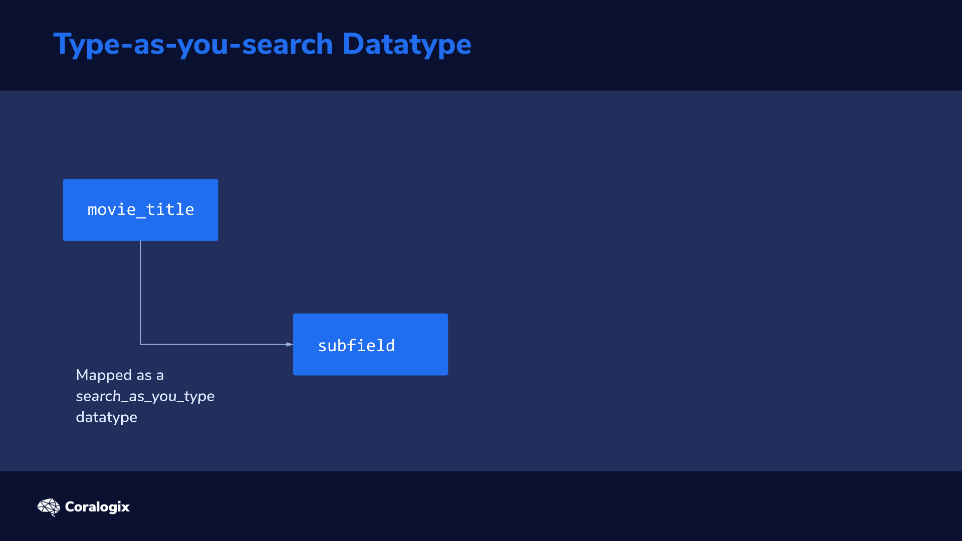
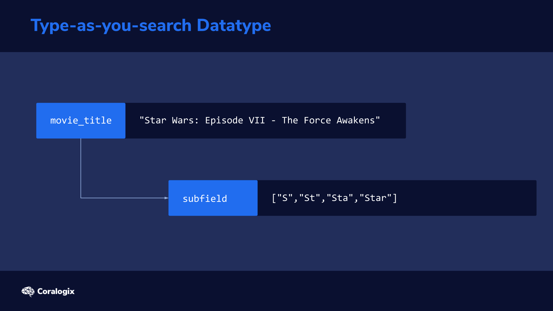
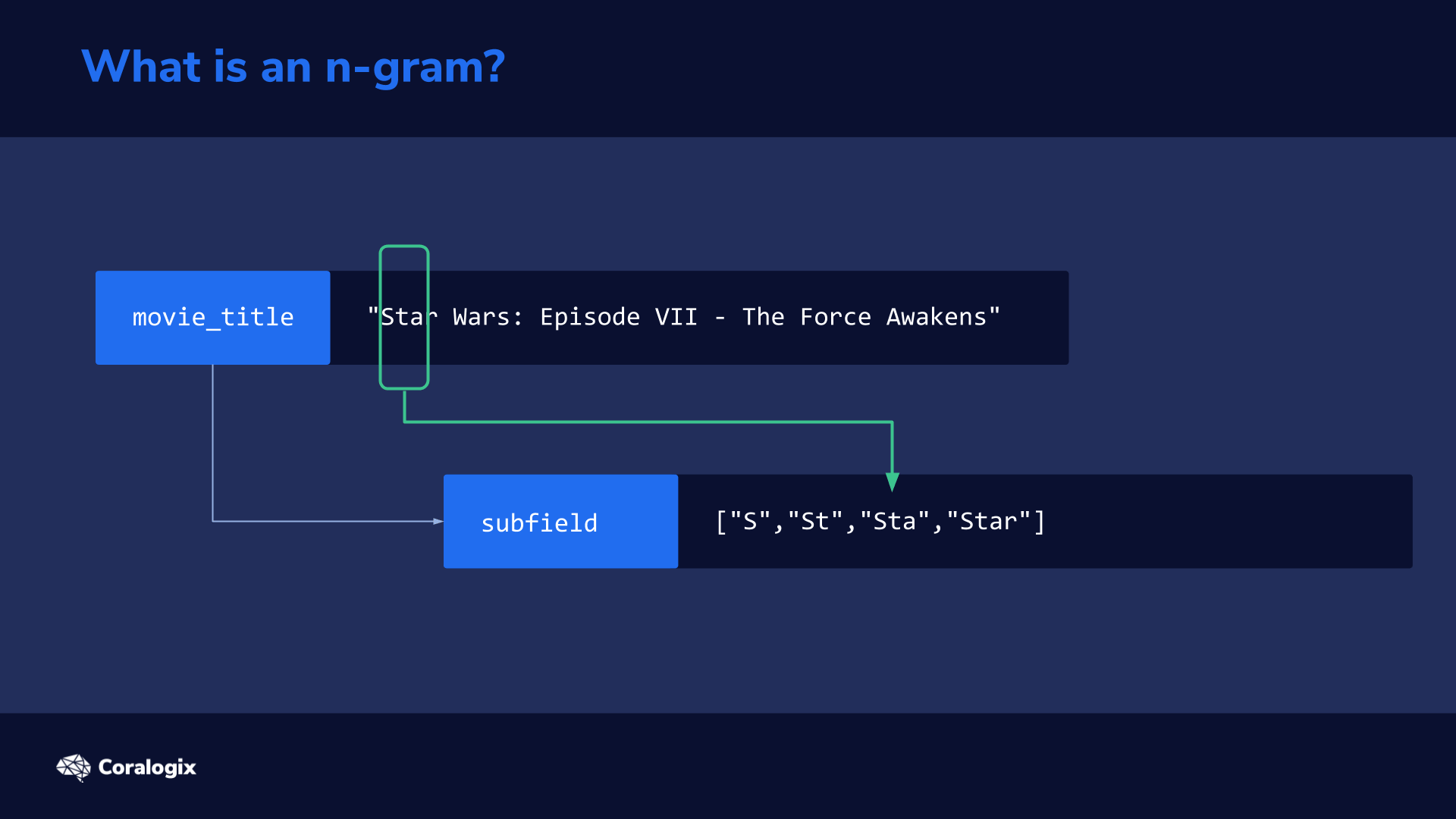
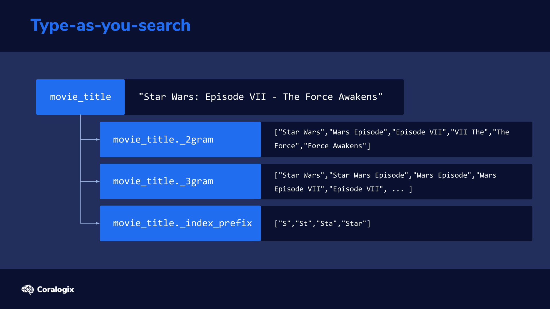


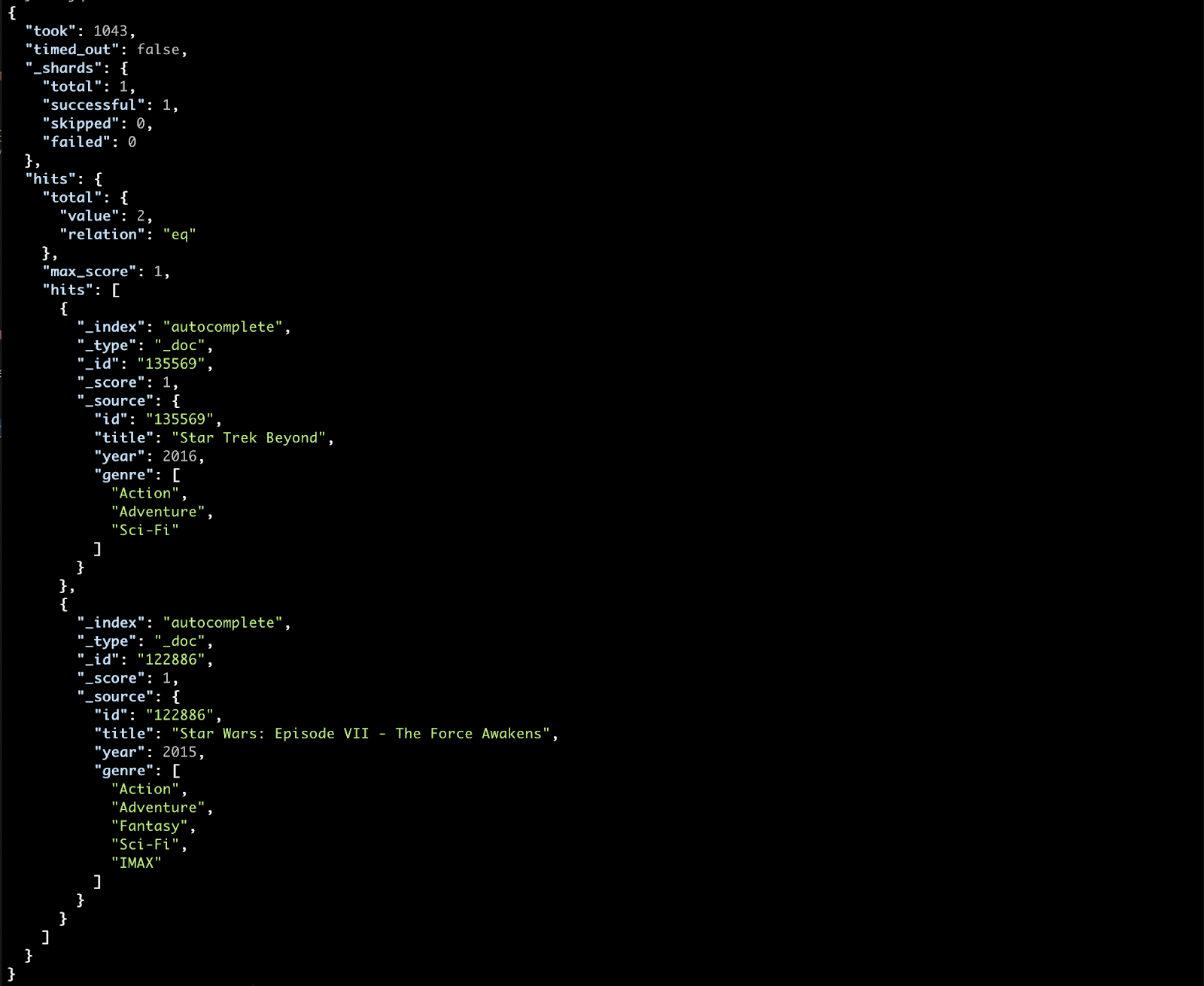


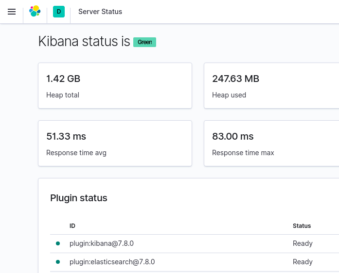
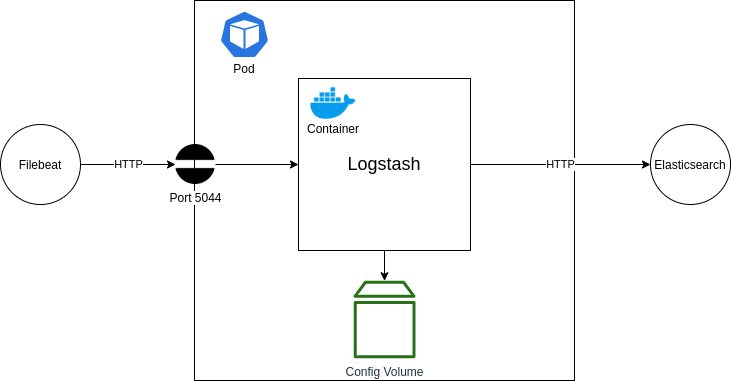
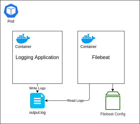
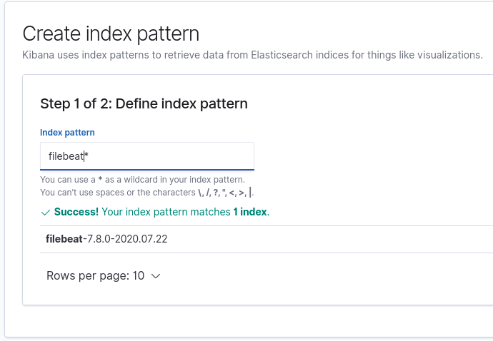
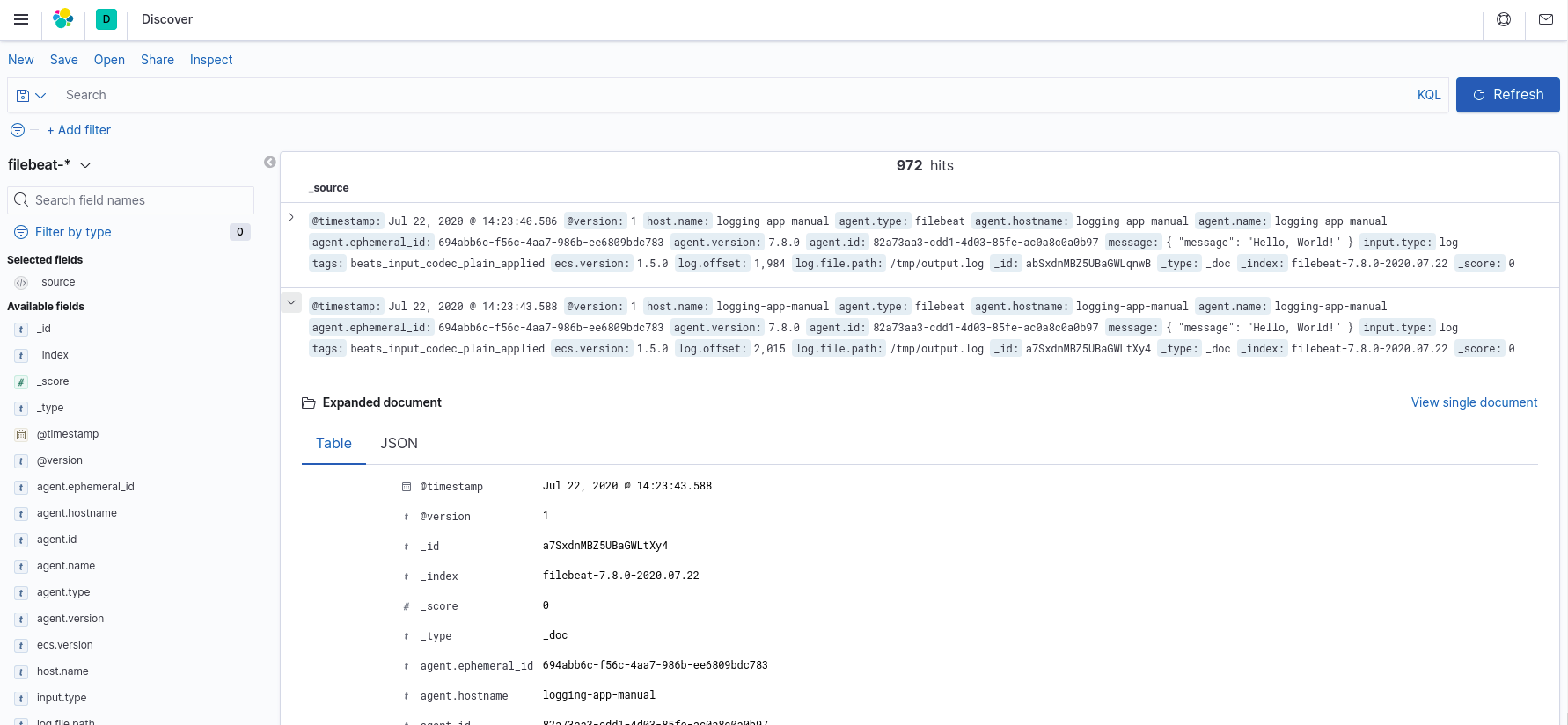

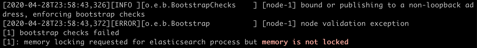


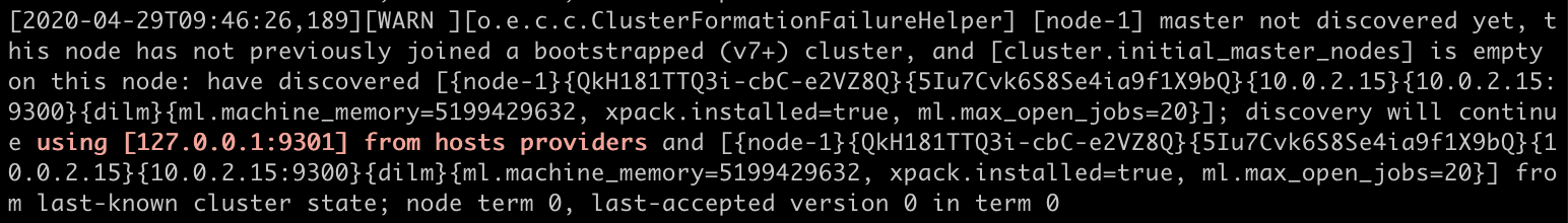
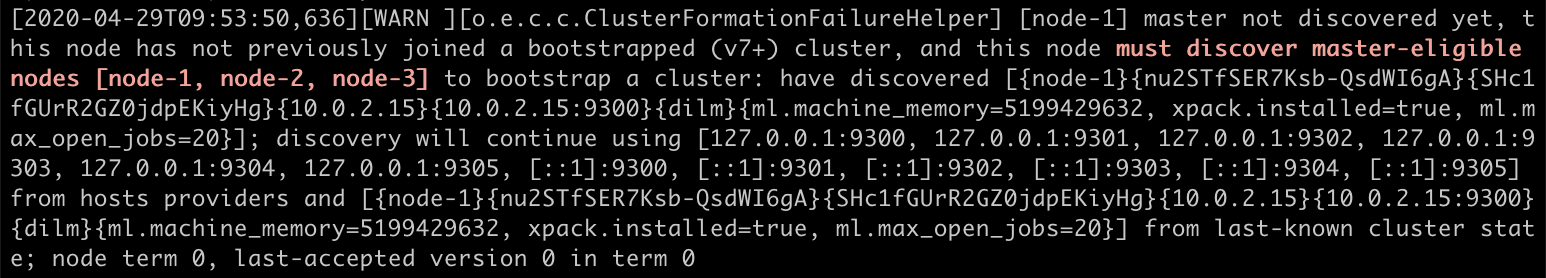

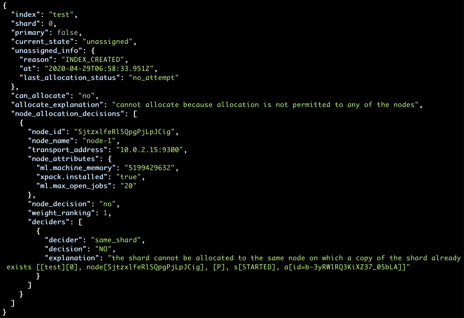

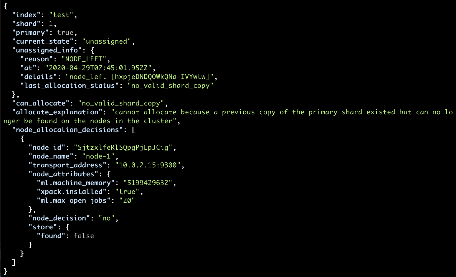
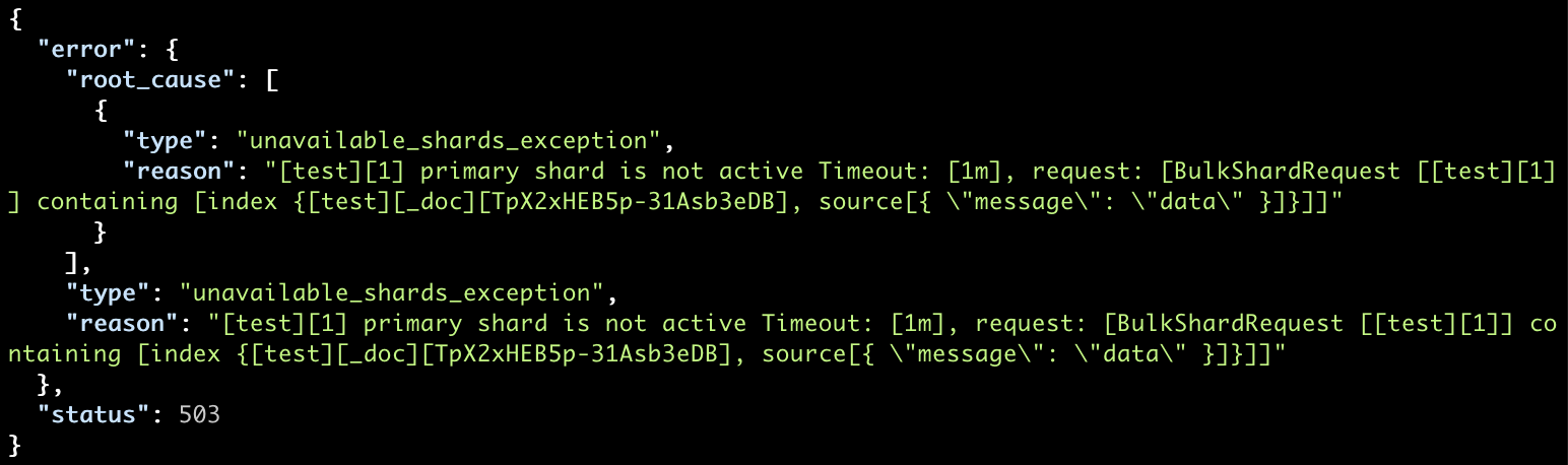

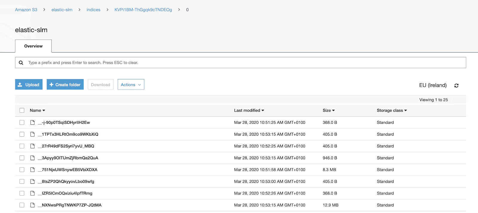
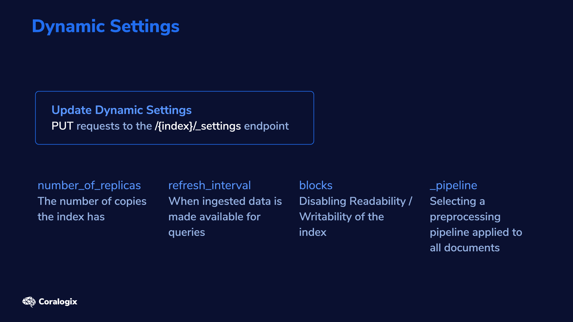
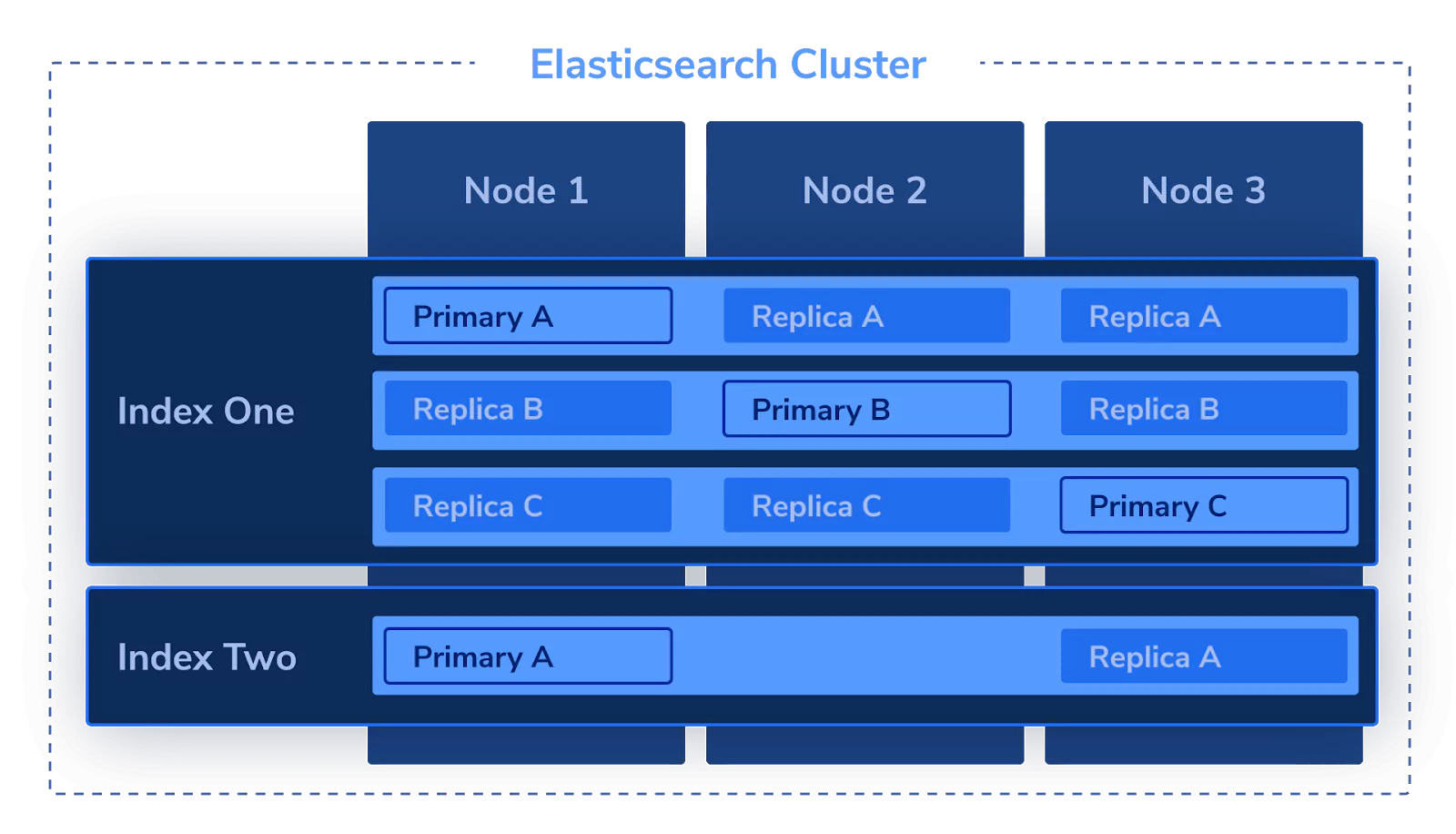
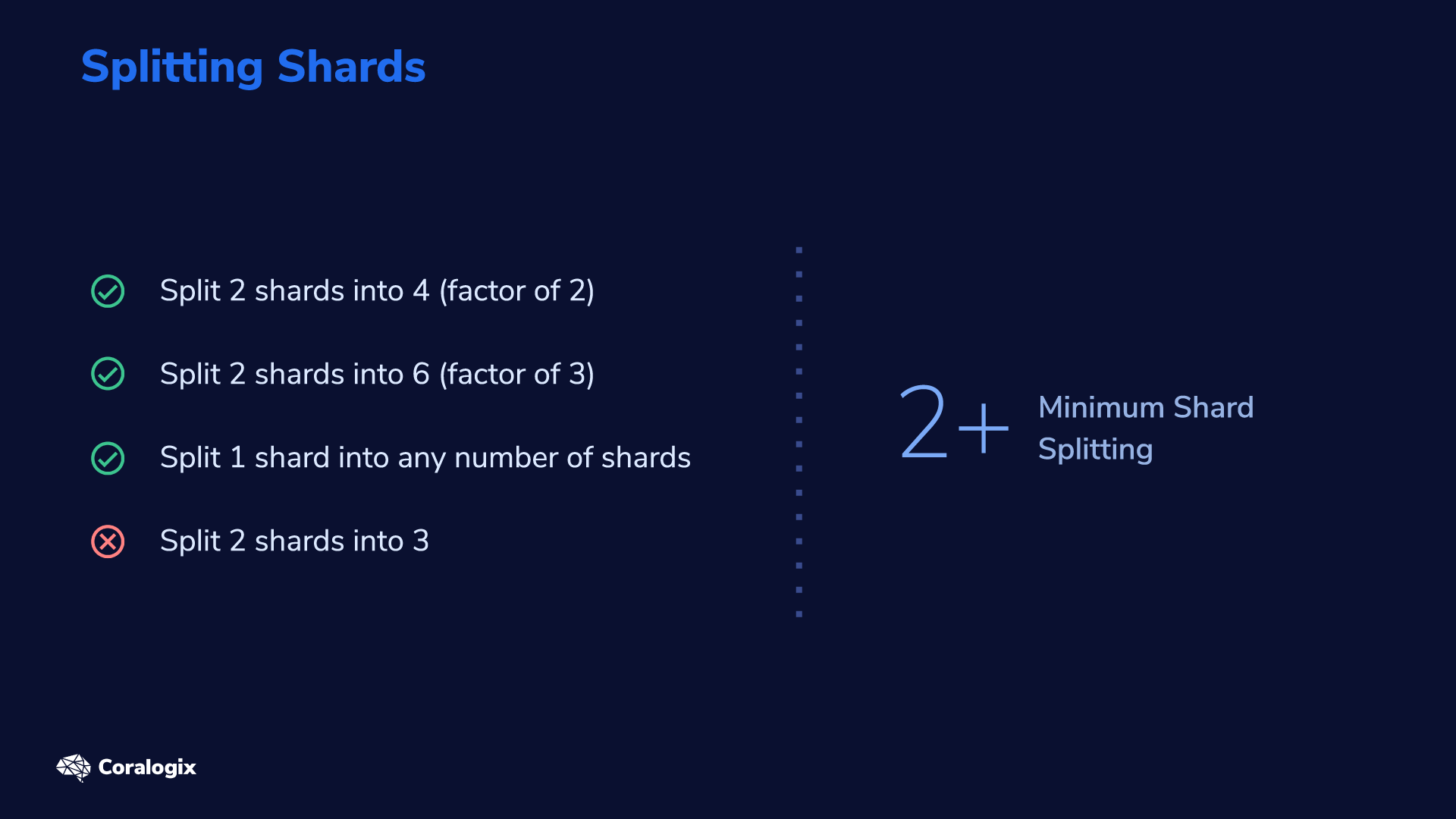
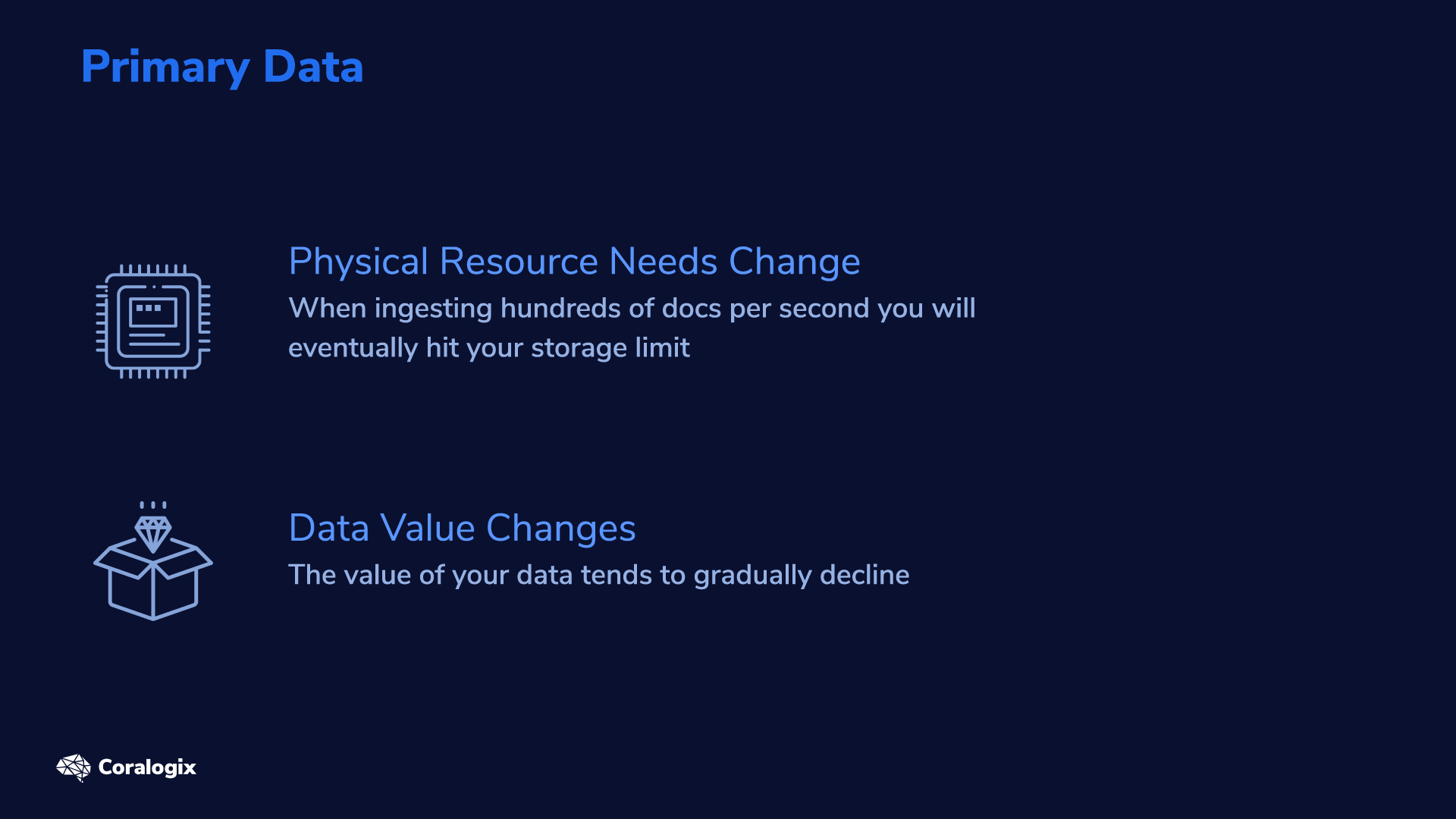 When you change your primary index data there aren’t many ways to reconstruct it. Now, you may be thinking, “why change the primary data at all?”
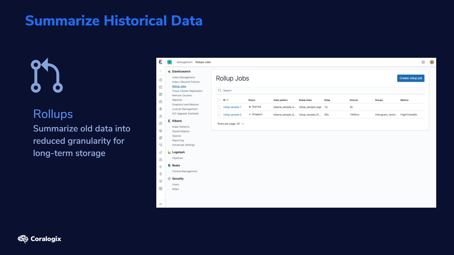

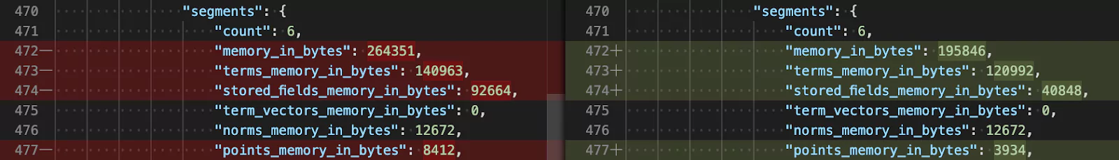
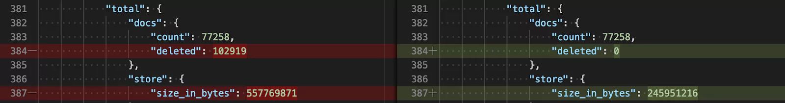

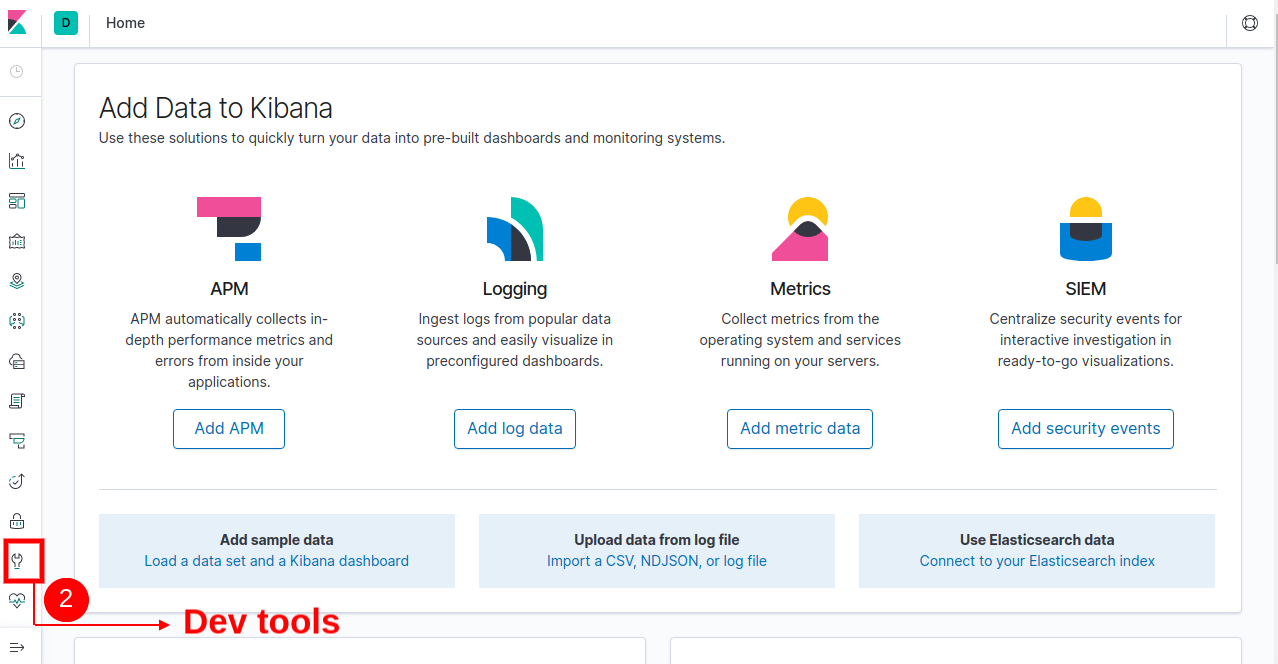
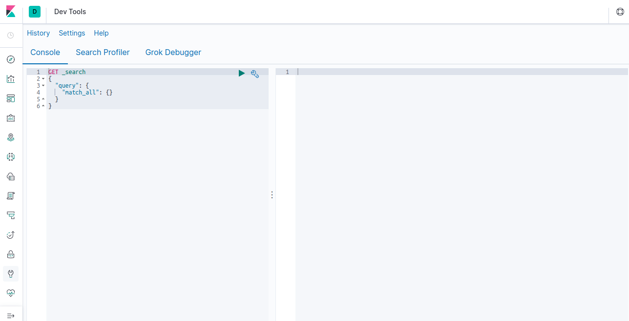
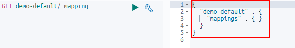
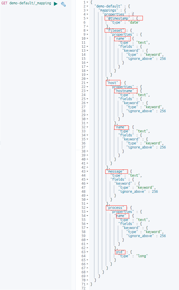
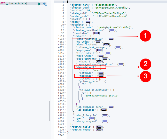
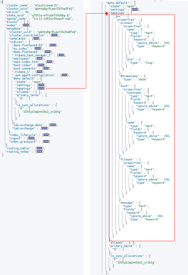
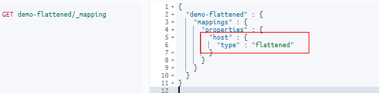
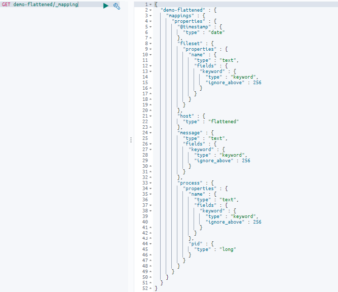
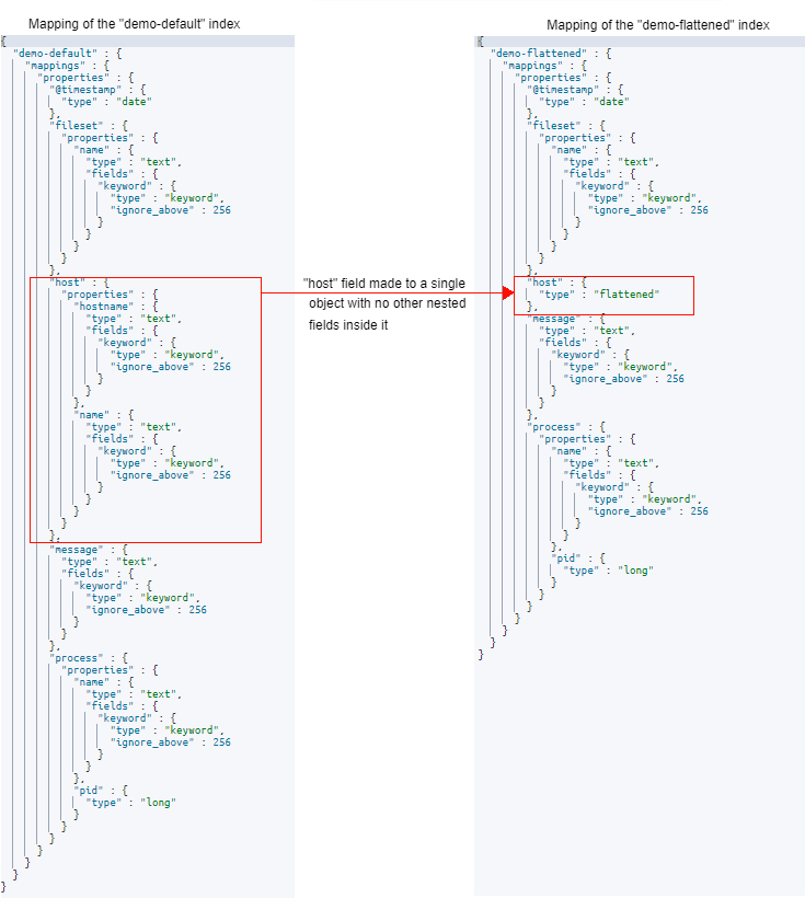
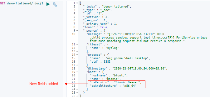
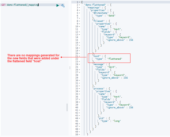
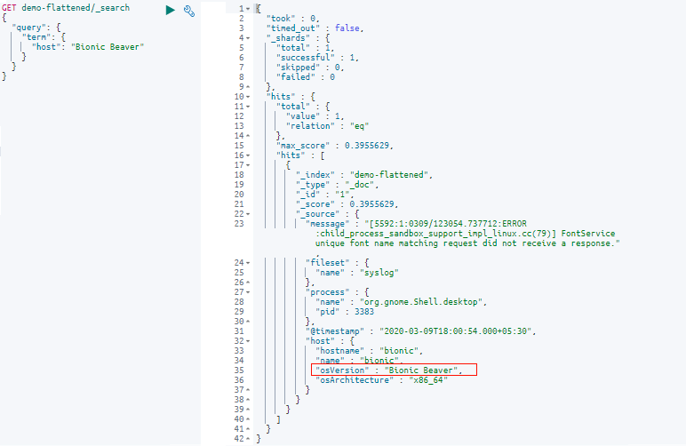
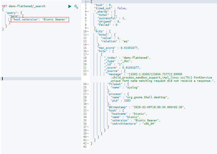
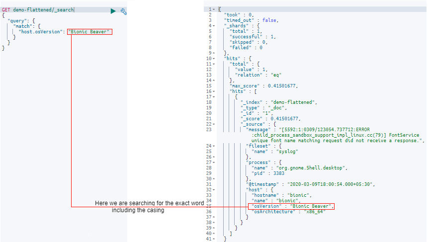
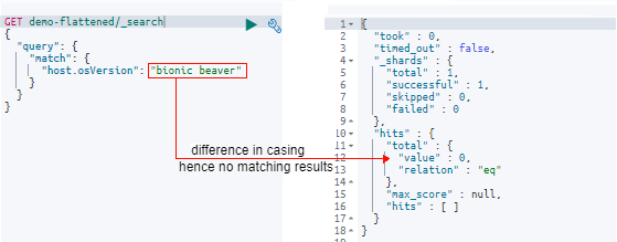
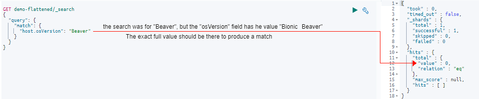
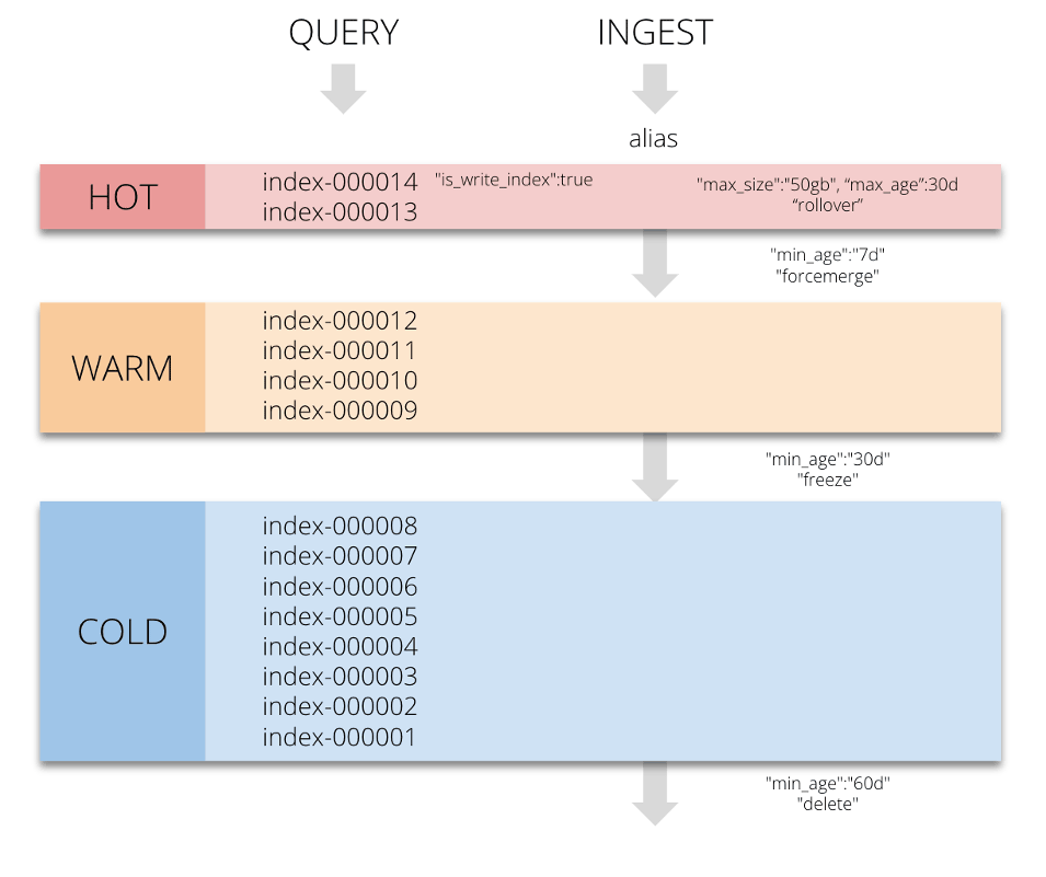 To achieve this we need to be able to automatically and continually move the shards between nodes that have different resource characteristics based on preset conditions. For example, placing shards of a newly created index on HOT nodes with SSDs and then after 14 days, moving those shards away from the HOT nodes to long term storage to make space for fresher data on the more performant hardware). There are three complementary Elasticsearch instruments that come handy for this situation: