Grafana is a popular way of monitoring and analysing data. You can use it to build dashboards for visualizing, analyzing, querying, and alerting on data when it meets certain conditions.
In this post, we’ll look at an overview of integrating data sources with Grafana for visualizations and analysis, connecting NoSQL systems to Grafana as data sources, and look at an in-depth example of connecting MongoDB as a Grafana data source.
MongoDB is a document or a document-oriented database and the most popular database for modern apps. It’s classified as a NoSQL system, using JSON-like documents with flexible schemas. As one of the most popular NoSQL databases around, and the go-to tool for millions of developers, we will focus on this to begin with, as an example.
General NoSQL via Data Sources
What is a data source?
For Grafana to play with data, it must first be stored in a database. It can work with several different types of databases. Even some systems not primarily designed for data storage can be used.
Grafana data source denotes any location wherein Grafana can access a repository of data. In other words, Grafana does not need to have data logged directly into it for that data to be analyzed. Instead, you can connect a data source with the Grafana system. Grafana then extracts that data for analysis, divinating insights and doing essential monitoring.
How do you add a data source?
To add a data source in Grafana, hover your mouse over the gear icon on the top right, (the configuration menu) and select the Data Sources button:
Once in that section, click the Add data source button. This is where you can view all of your connected data sources. You will also see a list of officially supported types available to be connected:
Once you’ve selected the data source you want, you will need to set the appropriate parameters such as authorization details, names, URL, etc.:
Here you can see the Elasticsearch data source, which we will talk about a bit later. Once you have filled the necessary parameters, hit the Save and Test button:
Grafana is going to now establish a connection between that data source and its own system. You’ll be given a message letting you know when this connection is complete. Then head to the Dashboards section in Grafana to begin venturing through that connected data source’s data.
Elasticsearch
This can function as both a logging and document-oriented database. Use Elasticsearch for powerful search engine capabilities or as a NoSQL database that can be connected directly with Grafana.
Let’s head back to the stage that appears after you click the button Add data source. When the list of available and officially supported data sources pops up, scroll down to the bit that says “Find more data source plugins on Grafana.com”:
This link will lead to a page of available plugins (make sure that the plugin type selected is data source, on the left-hand menu):
Plugins that are officially supported will be entitled “by Grafana Labs”, while open-source community plugins will have the individual names of developers:
Selecting any of the options will take you to a page with details about the plugin and how to install. After installation, you should see that data source in your list of available data sources in the Grafana UI. If you’re still unclear, there is a more detailed instruction page.
Make a Custom Grafana Data Source
You have the option to make your own data source if there isn’t appropriate one in the official list or community-supported ones. You can make a custom plugin for any database you prefer as long as it uses the HTTP protocol for client communications. The plugin needs to modify data from the database into time-series data so that Grafana can accurately represent in its dashboard visualisations.
You need these three aspects in order to develop a product plugin for the data source you wish to use:
QueryCtrl JavaScript class (allows you to do metric edits in dashboards panels)
ConfigCtrl JavaScript class (configure your new data source, or user-edit)
Data source JavaScript object (handles comms between the data source and data transformation)
MongoDB as a Grafana Data Source — The Enterprise Plugin
NoSQL databases handle enormous amounts of information vital for application developers, SREs, and executives — they get to see real-time infographics.
This can make them a shoe-in with regards to growing and running businesses optimally. See the plugin description here, entitled MongoDB Datasource by Grafana Labs.
MongoDB was added as a data source for Grafana around the end of 2019 as a regularly maintained plugin.
Setup Overview
Setting a New Data Source in Grafana
Make sure to name your data source Prometheus (scaling Prometheus metrics) so that it is by default identified by graphs.
Configuring Prometheus
By default Grafana’s dashboards work with the native instancetag to sort through each host, it is best to use a good naming system for each of your instances. Here are a few examples:
The names that you give to each job is not the essential part. But the ‘Prometheus’ dashboard will take Prometheusas the name.
Doing Exports
The following are the baseline option sets for the 3 exporters:
mongodb_exporter: sticking with the default options is good enough.
Grafana 5.x or later, make mysqld_export.yml here:
/var/lib/grafana/conf/provisioning/dashboards
with the following content:
Restarting Grafana:
Finally:
service grafana-server restart
Patch for Grafana 3.x
For users of this version a patch is needed for your install in order to let the zoomable graphs be accessible.
Updating Instructions
You just need to copy your new dashboards to /var/lib/grafana/dashboards then restart Grafana. Alternatively you can re-import them.
What Do the Graphs Look Like?
Here are a few sample graphs.
Benefits of Using MongoDB Backend Database as Grafana Data Source
Using the Grafana MongoDB plug-in, you can quickly visualize and check on MongoDB data as well as diagnostic metrics.
Diagnose issues and create alerts that let you know ahead of time when adjustments are needed to prevent failures and maintain optimal operations.
For MongoDB diagnostics, monitor:
Network: data going in and out, request stats
Server connections: total connections, current, available
Memory use
Authenticated users
Database figures: data size, indexes, collections, so on.
Connection pool figures: created, available, status, in use
For visualizing and observing MongoDB data:
One-line queries: eg. combine sample and find, eg. sample_nflix.movies.find()
Quickly detect anomalies in time-series data
Neatly gather comprehensive data: see below for an example of visualizing everything about a particular movie such as the plot, reviewers, writers, ratings, poster, and so on:
Grafana has a more detailed article on this here. We’ve only scratched the surface of how you could use this synchronicity.
Continuous Integration and Continuous Delivery (CI/CD) delivers services fast, effectively, and accurately. In doing so, CI/CD pipelines have become the mainstay of effective DevOps. But this process needs accurate, timely, contextual data if it’s to operate effectively. This critical data comes in the form of logs and this article will guide you through optimizing logs for CI/CD solutions.
Logs can offer insight into a specific event in time. This data provides a metric that can be used to forensically identify any issue that could cause problems in a system. But logs, especially in modern, hyperconnected ecosystem-based services, require appropriate optimization to be effective. The development of logging has generated a new approach, one that works to optimize the data delivered by logs and in turn, create actionable alerts.
Structured Logs Are Actionable
JSON effectively adds “life to log data”. It’s an open-standard file format that allows data to be communicated across web interfaces. Data delivered using JSON makes it easy to visualize and easy to read.
It can be filtered, grouped, tagged by type, and labeled. These features make JSON perfect for building focused queries and filtering based on two or more fields or zeroing in on a range of values within a specific field. At the end of the day, this saves developers. Also, it’s straightforward to transform legacy data into JSON format, so it really is never too late.
The Importance of Log Severity
A definition of the severity of a log is important to standardize across the organization. These levels act as a baseline for understanding what actions should be taken. Typical levels of severity for logs are:
Debug: describes a background event. These logs are not usually needed except to add context and analysis during a crisis. These logs are also useful when tuning performance or debugging.
Info: logs that represent transaction data, e.g. a transaction was completed successfully.
Warning: these logs represent unplanned events, for example, they may show that an illegal character for a username was received but is being ignored by the service. These are useful to locate possible flaws in a system over time and allow changes to improve system usability, etc.
Error: represent failures in processes that may not materially affect the entire service. These logs are useful when aggregated and monitored to look for trends to help improve service issues.
Critical: these logs should trigger an immediate alert to take action. A fatal log implies a serious system failure that needs immediate attention. Typically, in a day, 0.01% of logs would be defined as high severity.
5 Logging Best Practices
Once severity definition is resolved there are a number of best practices that further enhance the effectiveness of logging. These best practices facilitate the optimization of a CI/CD pipeline.
Log communication between components
Services are often ecosystems of interconnected components. All events in the system, including those that happen across the barrier between components, should be logged. The event lifecycle should be recorded, that is what happens at each component as well as during communication between components.
Log communications with external APIs
The API economy has facilitated the extended service ecosystem. But API events often happen outside your own organization. Optimized logging records what is communicated across the API layer. For example, if your offering uses a service such as SendGrid to send out communication emails to users, you need to know if critical alert emails are being sent? If not, this would need to be addressed. Log everything up to the point of sending to an API as well as logging the response from the other component to achieve a comprehensive view.
Add valuable metadata to your log
Modern service ecosystems, many stakeholders need access to logs. This includes Business Intelligence teams, DevOps, Support engineers, etc. Logs should include rich metadata, e.g. location, service name, version, environment name, and so on.
Log accessibility
You may not be the only one reading the logs. As companies scale, often access is needed by other stakeholders to change code, etc. Centralizing the log data becomes a necessity.
Combine textual and metric fields
Improve snapshot understanding of logs by having explanatory text (e.g., “failed to do xxx”) combined with metadata fields to provide more actionable insights. This offers a way to look at logs to see an at-a-glance view of the issue before drilling into performance data.
The Art and Science of Alerts
Logs are a leading indicator of issues and can be used for more than a postmortem analysis. Whilst metrics for infrastructure only presents an outcome of problematic code/performance, logs are the first encounter with code in use. As such, logs offer an easy way to spot things before they are felt at the user end. This is key to CI/CD enhancement.
Logs need to be accurate and have context (unlike metrics). Being able to make alerts specific and contextual is a way to tease out greater intelligence from the alert. Classification of alerts is a way to ensure that your organization gets the most from alerts and does not overreach.
Types of logging alerts:
Immediate alert: These alerts point to a critical event and are generated from critical and fatal logs. They require immediate attention to fix a critical issue.
“More than” alert: Sent out if something happens more than a predefined number of times. For example, less than 1 in 1000 people are failing to pay; if greater than 10 users are failing to pay the alert is generated. If these types of alerts are properly defined and sent to the right channel they can be acted upon and be highly effective.
“Less than” alert: These tend to be the most proactive alert type. They are sent when something is NOT happening.
If these alerts are channeled correctly, have context, and can be interpreted easily, they will be actionable and useful.
Coralogix goes further and adds further granularity to alerts:
Dynamic alert: Set a dynamic threshold for criteria.
Ratio alert: Allows an alert based on a ratio between queries
Alert Structure
Classification of alerts is one criterion; another is the alert structure. This ensures that alerts go to the right person(s). For example, is using Slack to collate alerts, a dedicated area can be set up to collate logging and metrics. The alerts can be then be directed to specific teams – this technique also helps alleviate alert fatigue.
To Push or Not to Push an Alert
The decision to push, or not, an alert, is an important aspect of creating an effective ‘alert culture’. Ask yourself certain questions: How would you feel if you received a specific type of alert at 2 am? What would you do? If you would be angered by getting this alert at that time, don’t push it. If, instead, your reaction is to say, “I must look at this tomorrow”, define the alert on your dashboard, but DO NOT push it. If the reaction is to stop what you are doing and respond – push the alert.
This simple logic can go a long way to making alerts actionable and workable and ends up reducing alert fatigue and keeping the team happy.
Summary
Coralogix is a full-stack observability platform that will drastically reduce logging costs but also improve your ability to query, monitor, manage log data, and to extend the log data value even further by turning logs into long-term metrics. Start a conversation with our logging experts today by clicking on the chat button on the bottom right corner, or start a free trial.
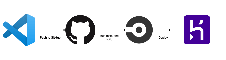
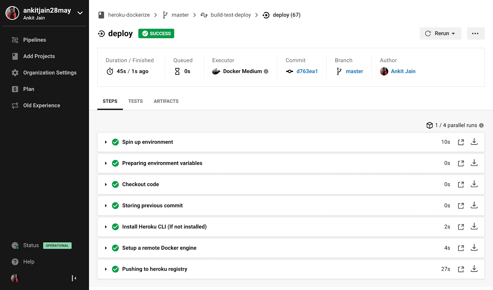
In this tutorial, we will be using Heroku to deploy our Node.js application through CircleCI using Docker. We will set up Heroku Continuous Integration and Deployment (CI/CD) solution pipelines using Git as a single source of truth.
Containerization allows developers to create and deploy applications faster with a wide range of other benefits like increased security, efficiency, agility to integrate with DevOps pipelines, portability, and scalability. Hence, companies and organizations are largely adopting this technology and it’s resulting in benefits for developers and removing overhead for the operations team in the software development lifecycle.
Benefits of having an Heroku CI/CD pipeline:
Improved code quality and testability
Faster development and code review
Risk mitigation
Deploy more often
Requirements
To complete this tutorial you will need the following:
The application architecture is always fundamental and important so we can properly align our various components in a systematic way to make it work. Let’s define the architecture of our example application so that we can have a proper vision before writing our code and integrating CI/CD pipelines.
We’ll be using Docker to deploy our Node.js application. Docker provides the flexibility to ship the application easily to cloud platforms. We will be using CircleCI as going to be our Heroku Continuous Integration and Deployment tool where we will run our unit and integrations tests. If tests are passed successfully, we are good to deploy our application on Heroku using Container Runtime.
Setup Application
Let’s start working on this by creating a small Node.js project. I’ve already created a small Node.js application that uses Redis to store key/value pairs. You can find the application on GitHub repo under the nodejs-project branch.
You can fork and clone the repo and setup Node.js application locally by running the following–
git clone -b nodejs-project https://github.com/ankitjain28may/heroku-dockerize.git
cd heroku-dockerize
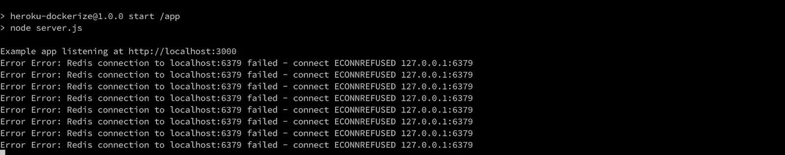
Our application uses Redis for storing key/values pairs so if you have Redis locally installed and running, we can test this application once locally before dockerizing it by running the following command:
npm start
# Output
> [email protected] start /heroku-dockerize
> node server.js

Example app listening at https://localhost:3000
Redis client connected
Let’s browse our application by opening the URL https://localhost:3000/ping in the browser. If we don’t have Redis configured locally, no problem, we have your back. We will be running this application using Docker Compose locally before pushing it to Git.
Dockerize Application
This is our own Node.js application and there is no Docker image available right now so let’s write our own by creating a file named `Dockerfile`.
FROM node:14-alpine

RUN apk add --no-cache --update curl bash
WORKDIR /app

ARG NODE_ENV=development
ARG PORT=3000
ENV PORT=$PORT

COPY package* ./
# Install the npm packages
RUN npm install && npm update

COPY . .

# Run the image as a non-root user
RUN adduser -D myuser
USER myuser

EXPOSE $PORT

CMD ["npm", "run", "start"]
We will be using an official node:14-alpine image from Dockerhub as our base image. We have preferred the alpine image because it’s minimal and lightweight as it doesn’t have additional system packages/libraries which we can always install on top of it using the package manager.
We have defined `NODE_ENV, PORT` as build arguments. We can install only the application dependencies by setting `NODE_ENV=production` while building an image for the production environment. This will install only the application dependencies leaving all the devDependencies.
Note: I am also running `npm update` along with `npm install`, it’s not generally a best practice to run `npm update` as it’s possible that it might break our application due to some updated dependencies while running in production which can result in downtime.
Also, we will be setting up our Heroku Continuous Integration pipeline where we will be running our integration tests and code linting where such issues can be caught before deploying our application.
Awesome! Let’s build our image using the following command:
Let’s check our image by running `docker images` command–
docker images
The output will be something similar as shown in the image below:
We can now run our application container using the image created above by running the following command:
docker run --rm --name heroku-dockerize -p 3000:3000 heroku-dockerize:local
We can see the output as shown in the image below–
Oops!!! We’ve dockerized our Node.js application but we haven’t configured Redis yet. We need to create another Docker container using the Redis official docker image and create a network between our application container and the Redis container.
Too many things to take care of, so here comes Docker Compose to help. Compose is a tool for defining and running multi-container applications with ease; removing the manual overhead of creating networks, attaching containers to the network, etc.
Let’s set up Docker Compose by creating a file named `docker-compose.yaml`
We have defined our two services named `web` for our Node.js application and `db` for our redis.
Add the following variables to the .env file
PORT=3000
REDIS_URL=redis://db:6379
It is always recommended to store the sensitive values or credentials in `.env` file and add this file in `.gitignore` and `.dockerignore` so we can restrict its circulation.
Let’s create a `.gitignore` and `.dockerignore` file and add the following–
node_modules
.env
.git
coverage
Awesome, Let’s spin our containers using docker-compose–
docker-compose up -d
We can check whether both services are up and running by running the following command —
docker-compose ps
Let’s browse our application and make some dummy request to save data to our redis service.
curl -X POST
      https://localhost:3000/dummy/1
      --header 'Content-Type: application/json'
      --data '{"ID":"1","message":"Testing Redis"}'
# Output
Successful
We have successfully saved our data in our redis, Let’s make a get request to `/dummy/1` to check our data–
curl -X GET https://localhost:3000/dummy/1
#Output
{"ID":"1","message":"Testing Redis"}
Note: We can use Postman to make an API request.
Before moving forward, let’s discuss the pros and cons of Heroku Container Runtime
Heroku Container Runtime
Heroku traditionally uses the Slug Compiler which compresses our code, creates a “slug” and distributes it to the dyno manager for execution. This is a very common understanding of what Slug Compiler does. With the increase in the adoption of Containerization and the benefits of it, Heroku has also announced Heroku Container Runtime which allows us to deploy our Docker images.
With Heroku Container Runtime, we can have all the benefits of Docker like the isolation of our application from the underlying OS, increased security, flexibility to create our custom stack. With Docker, we have an assurity that the application running inside the container on our local machines will surely run on the cloud/other machines, as the only difference between them is of the environment i.e config files or environment variables.
“With great powers come great responsibility”
Similar to this popular quotes, We have more responsibility to maintain and upgrade our Docker image, fixing any security vulnerability, unlike the traditional slug compiler. Other than that, Heroku Container Runtime is not yet mature as it doesn’t support most of the cool features of Docker. These are some of the major missing features that we use with Docker —
Volume Mounts is not supported and the filesystem is ephemeral.
Networking linking across dynos is not supported.
Only the web process (web dyno) is exposed to traffic and PORT is dynamically set by Heroku during runtime as an environment variable so an application must listen to that port, else it will fail to run.
It doesn’t respect the EXPOSE command in Dockerfile.
We will be using Heroku Container Runtime for deploying our application along with Heroku Manifest. With Heroku manifest, we can define our Heroku app and set up addons, config variables, and structure our images to be built and released.
As we are using Redis to store key/value pairs, we can define the Heroku Redis add-ons. Under the `setup` field, we can create global configurations and add-ons. Under the `build` field, we have defined our process name and the Dockerfile used to build our Docker image. We can also pass build arguments to our Dockerfile under the `config` field. We haven’t used the `release` field as we are not running any migrations or pre-release tasks. Finally, we have defined our dyno and command to be executed in the `run` field.
Note: If we don’t define the `run` field, the CMD command provided in Dockerfile is used.
Let’s create our app on Heroku. Hope you have installed the Heroku CLI and installed the `@heroku-cli/plugin-manifest` plugin. If not, please refer to this doc.
Run the following command to create our app from Heroku manifest file with all the add-ons and config variables–
Awesome, we have created our app on Heroku, it has also set our stack to a container. Let’s move to the next section and create our CI/CD pipeline to deploy our Node.js Application.
Heroku Continuous Integration
Continuous Integration (CI) is the process of automating the build and running all our test suites including unit tests, integration tests and also performs code validations and linting to maintain the code quality. If our code successfully passes all the checks and tests, it is good to be deployed to production.
We will be using CircleCi for creating our Heroku CI/CD pipelines. CircleCi is the cloud-based tool to automate the integration and deployment process. Heroku also offers CI/CD pipeline but as we discussed above, Heroku Container Runtime is not very mature and still under development and hence, it is not possible to test container builds via Heroku CI. We can use other third-party CI/CD tools like Travis, GitHub Actions etc.
CircleCI is triggered whenever we make a push event to the GitHub repo via webhooks. We can control the configure the webhooks to be triggered on different events like push, pull requests etc. CircleCI looks for the `.circleci/config.yml` file which contains the instructions/commands to be processed. Let’s create a `.circleci/config.yml` file–
CircleCI has recently introduced reusable packages written in YAML called “Orbs” to help developers with setting up their CI/CD pipeline easily and efficiently. It also allows us to integrate third-party tools effectively in our pipelines. In the above CircleCI config, we have used one such orb called `circleci/node` to easily install Node.js and its package manager.
We have set up the CI pipeline to build and test our application, it will first install the application dependencies and then run all our integration tests. We have also added the step to create the Docker image so we can check for our Docker image.
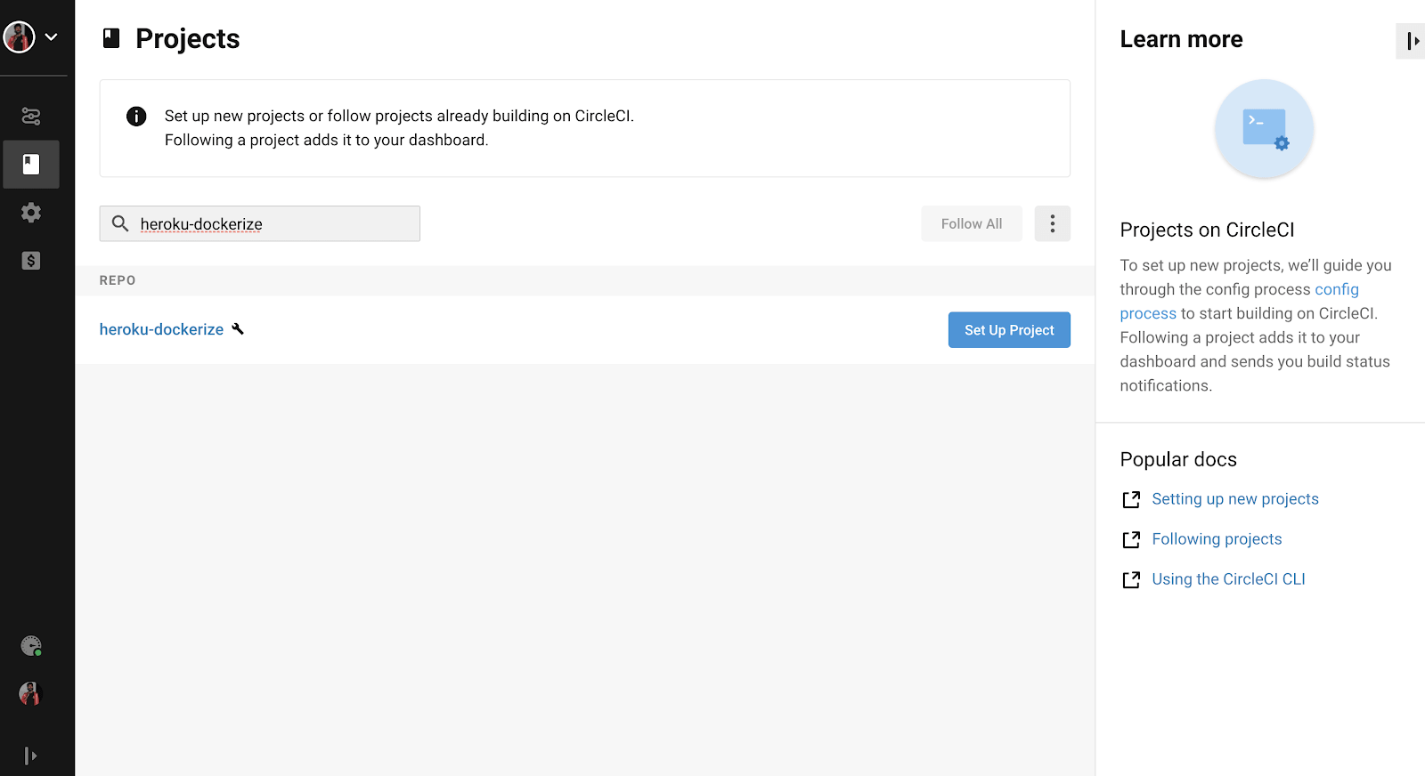
Let’s push this CircleCI config to our GitHub repo by running the following command–
We will now enable this repo from our CircleCI dashboard simply by clicking “Set Up Project” button as shown in the image below–
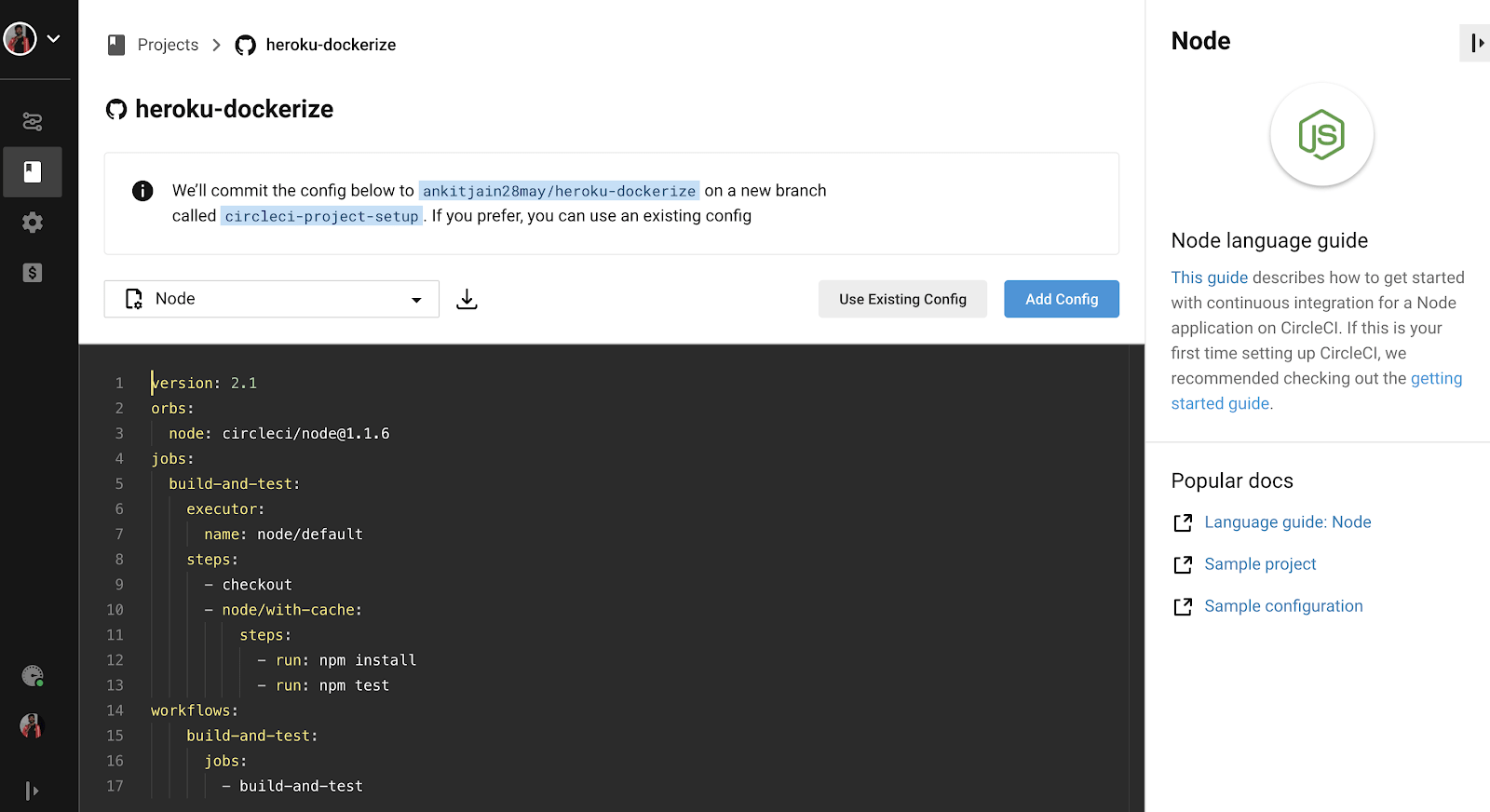
Once we click on this button, it will ask us to add a config file as shown in the image below:
Click on the “Use Existing Config” button as we have already added the CircleCI config and click on “Start Building”. It will start the build for your Node.js application. We can also run pre-tests scripts or post-tests script simply by adding another pre/post-run field.
Awesome, all tests were passed; we are good to deploy this application to our Heroku. Let’s move to our next step of integrating the CD pipeline to deploy this project to our Heroku application.
Integrating The CD Pipeline
In the previous step, we have configured our CI pipeline to make the builds and run all the tests so it can be deployable to the production environment. CI pipelines help the reviewers to review the code easily as all the tests are passed. It also allows the developers to have better visibility in the application code if something breaks without being blocked at the other developers to review.
Let’s deploy our application to Heroku by running the following command–
# deploy on Heroku
$ git push heroku master

# Open the website
$ heroku open

# Check the logs
$ heroku logs -a heroku-dockerize
Heroku has this great feature of deploying applications directly using Git. As we can see this is being done manually by us and it’s never good to deploy our application to production environments without running proper tests and reviews. Let’s add our CD pipeline.
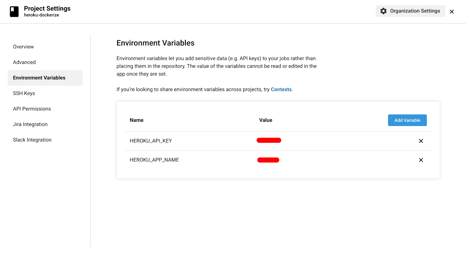
Before adding the pipeline, we need to authenticate the request which CircleCI makes to deploy our application on Heroku. This can be done by setting these two environment variables–
HEROKU_APP_NAME: Name of our Heroku app.
HEROKU_API_KEY: This is our Heroku API key which will serve as the token for authentication and verifies our request.
We can find the API Key under the Heroku Account Settings.
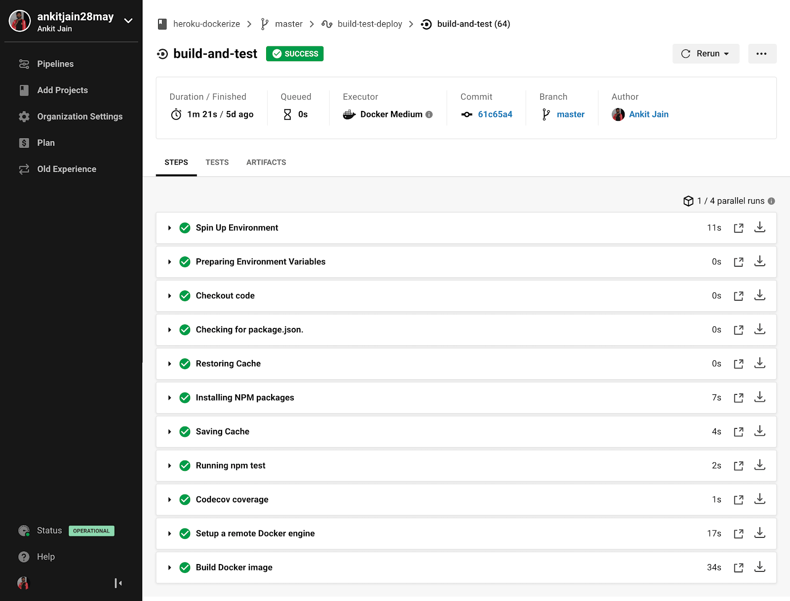
Let’s add them as Environment Variables in our CircleCI Project Settings Page as shown in the image below.
Open the `.circleci/config.yml` file and setup the deploy pipeline —
We are now using circleci/heroku orb to install Heroku CLI and deploy the application. We can also see that this orb supports the deploy-via-git command to deploy our application as we did above manually, but still, we are login to Heroku container registry and deploying our images. This is because we have run a pre-script to create a `/commit` endpoint which shows the deployed commit by rendering the data from `commit.txt` file.
Under workflows, we have made sure that our code is only deployed for the `master` branch and provided that `build-and-test` pipeline i.e our CI pipeline should be run successfully.
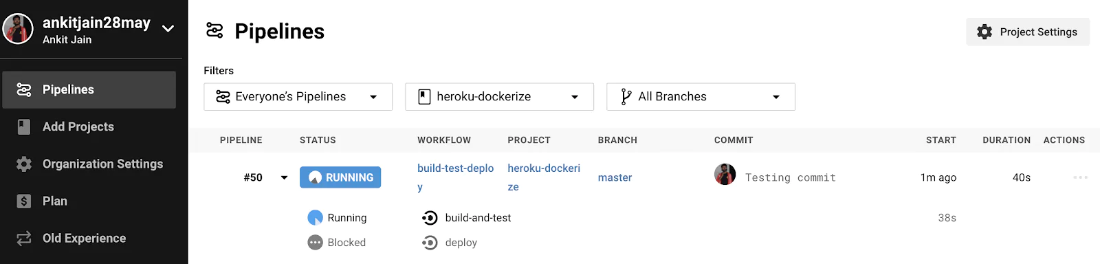
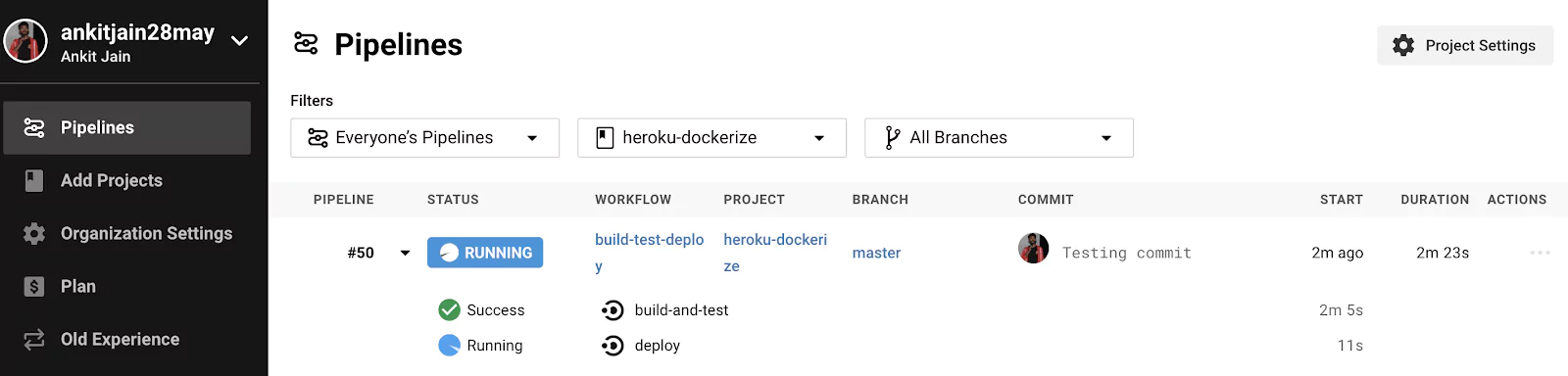
Let’s push our code with the Continuous Deployment configuration added to our CircleCI configuration. Our build will start to run as soon as we push. Let’s check the build–
Our pipeline is running and waiting for the CI pipeline (build-and-test) to be run successfully. Once CI pipeline is finished with success, Our CD pipeline (deploy) will run and deploy our application on Heroku.
Great, Our CD pipeline is working perfectly. Let’s open our application and check for the `/commit` endpoint as well as we can also verify our application’s other endpoint like saving data to Redis as a key/value pair. Browse the application at https://heroku-dockerize.herokuapp.com
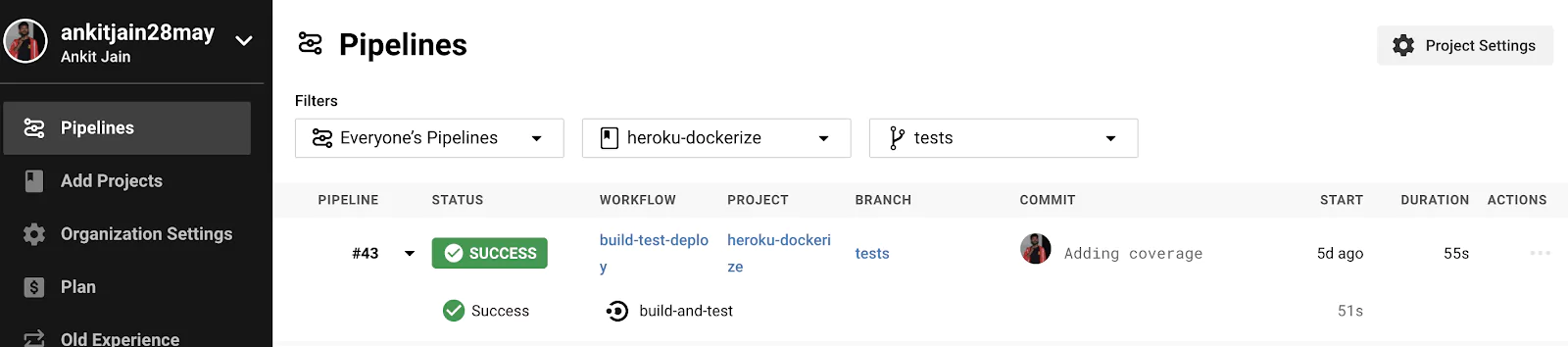
We have added the coverage and some extra tests under the `tests` branch which is merged to master now.
As we can see that it has skipped the CD pipeline (deploy) and only ran the CI pipeline (build-and-test). This is because we have defined that CD will run only for the master branch once the CI pipeline runs successfully. You can check the PR here #3
Conclusion
In this post, we first understand how we can dockerize our application and set up our local development environment using docker-compose. Further, we learned about the Heroku Container Runtime and how we can use it to automate the process of deploying our containerized applications to Heroku by using the Continuous Integration & Deployment pipeline. It will eventually increase the productivity of developers and help the teams to deploy their projects easily.
The code is available in this Github repo. The repo also contains the integration with Travis CI under `.travis.yml` file if anyone is willing to integrate it with Travis.
In this article, we’ll learn about the Elasticsearch flattened datatype which was introduced in order to better handle documents that contain a large or unknown number of fields. The lesson examples were formed within the context of a centralized logging solution, but the same principles generally apply.
By default, Elasticsearch maps fields contained in documents automatically as they’re ingested. Although this is the easiest way to get started with Elasticsearch, it tends to lead to an explosion of fields over time and Elasticsearch’s performance will suffer from ‘out of memory’ errors and poor performance when indexing and querying the data.
This situation, known as ‘mapping explosions’, is actually quite common. And this is what the Flattened datatype aims to solve. Let’s learn how to use it to improve Elasticsearch’s performance in real-world scenarios.
2. Why Choose the Elasticsearch Flattened Datatype?
When faced with handling documents containing a ton of unpredictable fields, using the flattened mapping type can help reduce the total amount of fields by indexing an entire JSON object (along with its nested fields) as a single Keyword field.
However, this comes with a caveat. Our options for querying will be more limited with the flattened type, so we need to understand the nature of our data before creating our mappings.
To better understand why we might need the flattened type, let’s first review some other ways for handling documents with very large numbers of fields.
2.1 Nested DataType
The Nested datatype is defined in fields that are arrays and contain a large number of objects. Each object in the array would be treated as a separate document.
Though this approach handles many fields, it has some pitfalls like:
Nested fields and querying are not supported in Kibana yet, so it sacrifices easy visibility of the data
Each nested query is an internal join operation and hence they can take performance hits
If we have an array with 4 objects in a document, Elasticsearch internally treats it as 4 different documents. Hence the document count will increase, which in some cases might lead to inaccurate calculations
2.2 Disabling Fields
We can disable fields that have too many inner fields. By applying this setting, the field and its contents would not be parsed by Elasticsearch. This approach has the benefit of controlling the overall fields but;
It makes the field a view only field – that is it can be viewed in the document, but no query operations can be done.
It can only be applied to the top-level field, hence need to sacrifice the query capability of all its inner fields.
The Elasticsearch flattened datatype has none of the issues that are caused by the nested datatype, and also provide decent querying capabilities when compared to disabled fields.
3. How the Flattened Type Works
The flattened type provides an alternative approach, where the entire object is mapped as a single field. Given an object, the flattened mapping will parse out its leaf values and index them into one field as keywords.
In order to understand how a large number of fields affect Elasticsearch, let’s briefly review the way mappings (i.e schema) are done in Elasticsearch and what happens when a large number of fields are inserted into it.
3.1 Mapping in Elasticsearch
One of Elasticsearch’s key benefits over traditional databases is its ability to adapt to different types of data that we feed it without having to predefine the datatypes in a schema. Instead, the schema is generated by Elasticsearch automatically for us as data gets ingested. This automatic detection of the datatypes of the newly added fields by Elasticsearch is called dynamic mapping.
However, in many cases, it’s necessary to manually assign a different datatype to better optimize Elasticsearch for our particular needs. The manual assigning of the datatypes to certain fields is called explicit mapping.
The explicit mapping works for smaller data sets because if there are frequent changes to the mapping and we are to define them explicitly, we might end up re-indexing the data many times. This is because, once a field is indexed with a certain datatype in an index, the only way to change the datatype of that field is to re-index the data with updated mappings containing the new datatype for the field.
To greatly reduce the re-indexing iterations, we can take a dynamic mapping approach using dynamic templates, where we set rules to automatically map new fields dynamically. These mapping rules can be based on the detected datatype, the pattern of field name or field paths.
Let’s first take a closer look at the mapping process in Elasticsearch to better understand the kind of challenges that the Elasticsearch flattened datatype was designed to solve.
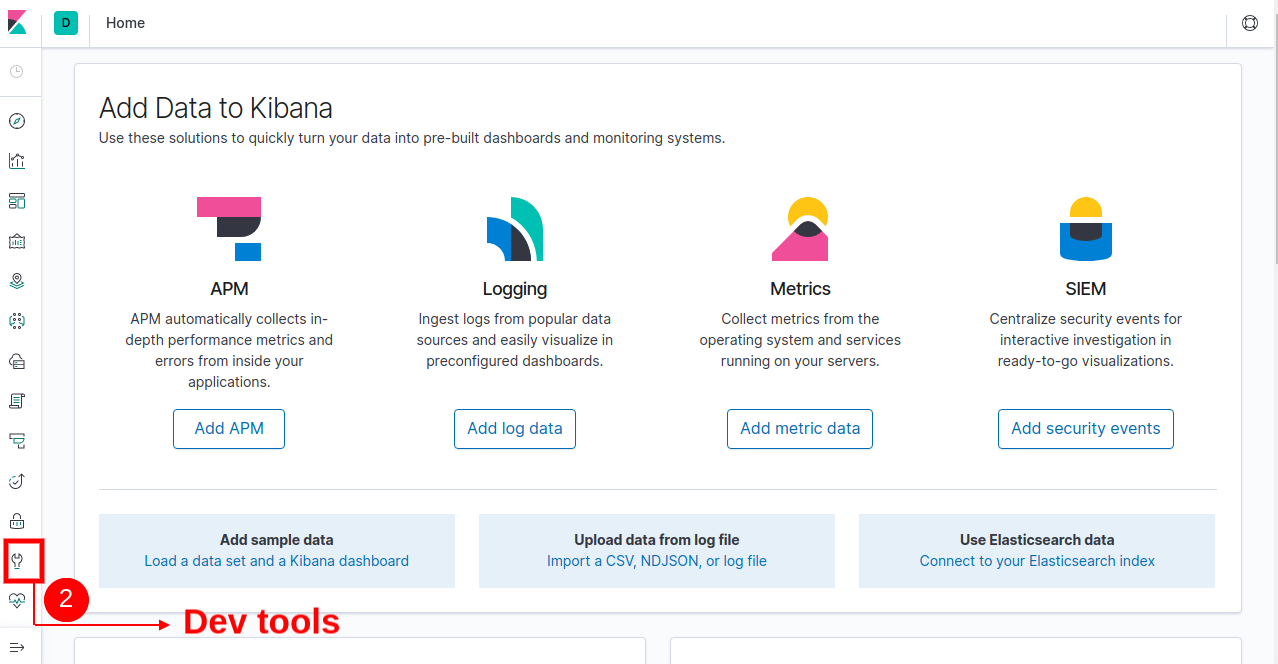
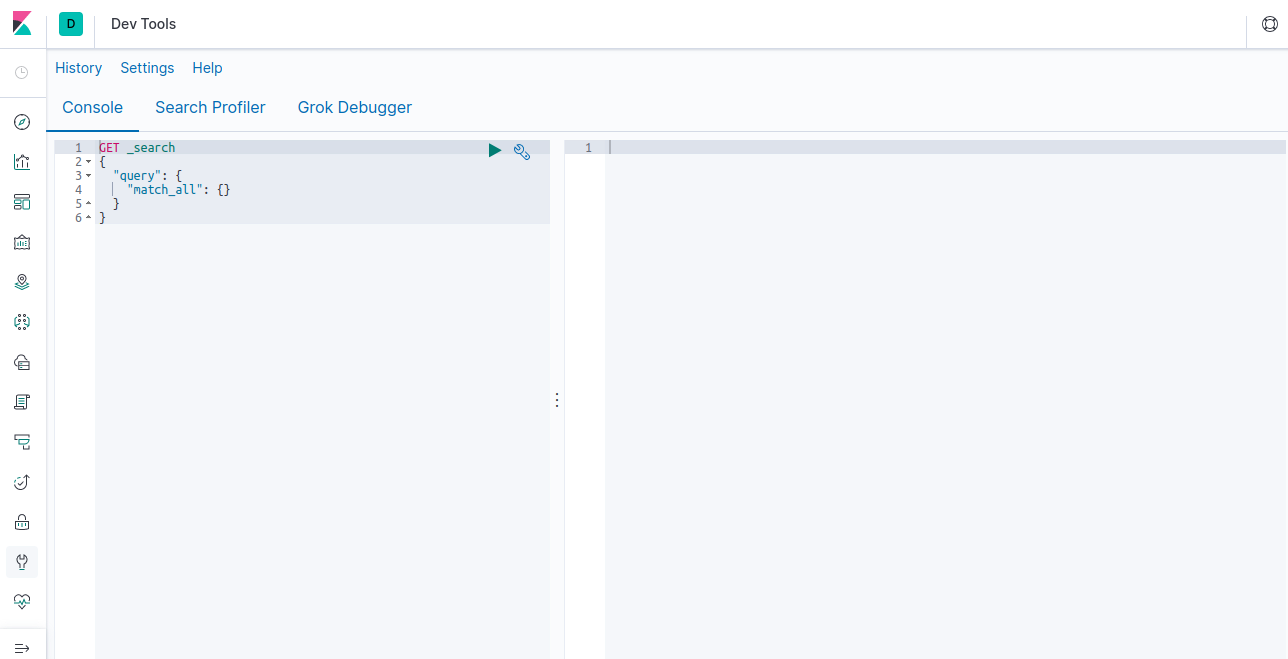
First, let’s navigate to the Kibana dev tools. After logging into Kibana, click on the icon (#2), in the sidebar would take us to the “Dev tools”
This will launch with the dev tools section for Kibana:
Create an index by entering the following command in the Kibana dev tools
PUT demo-default
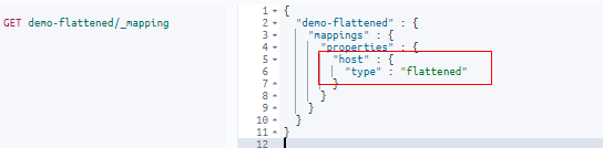
Let’s retrieve the mapping of the index we just created by typing in the following
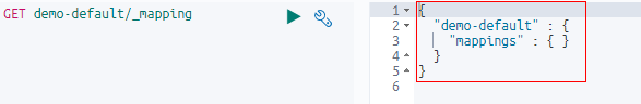
GET demo-default/_mapping
As shown in the response there is no mapping information pertaining to the index “demo-flattened” as we did not provide a mapping yet and there were no documents ingested by the index.
Now let’s index a sample log to the “demo-default” index:
PUT demo-default/_doc/1
{
  "message": "[5592:1:0309/123054.737712:ERROR:child_process_sandbox_support_impl_linux.cc(79)] FontService unique font name matching request did not receive a response.",
  "fileset": {
    "name": "syslog"
  },
  "process": {
    "name": "org.gnome.Shell.desktop",
    "pid": 3383
  },
  "@timestamp": "2020-03-09T18:00:54.000+05:30",
  "host": {
    "hostname": "bionic",
    "name": "bionic"
  }
}
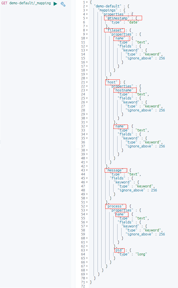
After indexing the document, we can check the status of the mapping with the following command:
GET demo-default/_mapping
As you can see in the mapping, Elasticsearch, automatically generated mappings for each field contained in the document that we just ingested.
3.2 Updating Cluster Mappings
The Cluster state contains all of the information needed for the nodes to operate in a cluster. This includes details of the nodes contained in the cluster, the metadata like index templates, and info on every index in the cluster.
If Elasticsearch is operating as a cluster (i.e. with more than one node), the sole master node will send cluster state information to every other node in the cluster so that all nodes have the same cluster state at any point in time.
Presently, the important thing to understand is that mapping assignments are stored in these cluster states.
The cluster state information can be viewed by using the following request
GET /_cluster/state
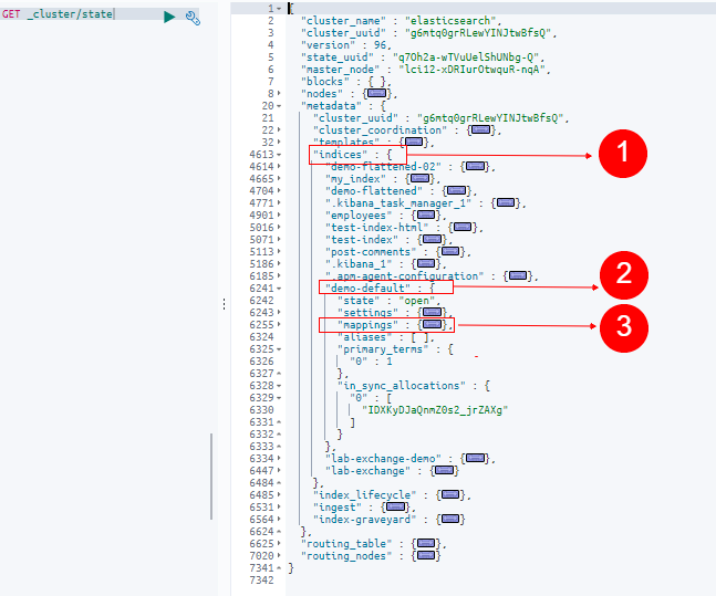
The response for the cluster state API request will look like this example:
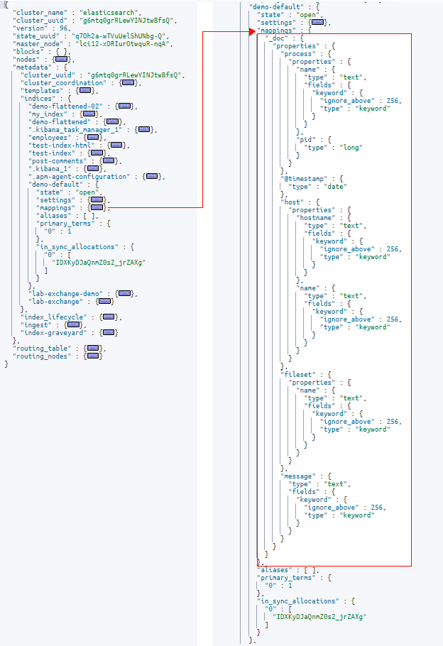
In this cluster state example you can see the “indices” object (#1) under the “metadata” field. Nested in this object you’ll find a complete list of indices in the cluster (#2). Here we can see the index we created named “demo-default” which holds the index metadata including the settings and mappings (#3). Upon expanding the mappings object, we can now see the index mapping that Elasticsearch created.
Essentially what happens is that for each new field that gets added to an index, a mapping is created and this mapping then gets updated in the cluster state. At that point, the cluster state is transmitted from the master node to every other node in the cluster.
3.3 Mapping Explosions
So far everything seems to be going well, but what happens if we need to ingest documents containing a huge amount of new fields? Elasticsearch will have to update the cluster state for each new field and this cluster state has to be passed to all nodes. The transmission of the cluster state across nodes is a single-threaded operation – so the more field mappings there are to update, the longer the update will take to complete. This latency typically ends with a poorly performing cluster and can sometimes bring an entire cluster down. This is called a “mapping explosion”.
This is one of the reasons that Elasticsearch has limited the number of fields in an index to 1,000 from version 5.x and above. If our number of fields exceeds 1,000, we have to manually change the default index field limit (using the index.mapping.total_fields.limit setting) or we need to reconsider our architecture.
This is precisely the problem that the Elasticsearch flattened datatype was designed to solve.
4. The Elasticsearch Flattened DataType
With the Elasticsearch flattened datatype, objects with large numbers of nested fields are treated as a single keyword field. In other words, we assign the flattened type to objects that we know contain a large number of nested fields so that they’ll be treated as one single field instead of many individual fields.
4.1 Flattened in Action
Now that we’ve understood why we need the flattened datatype, let’s see it in action.
We’ll start by ingesting the same document that we did previously, but we’ll create a new index so we can compare it with the unflattened version
After creating the index, we’ll assign the flattened datatype to one of the fields in our document.
Alright, let’s get right to it starting with the command to create a new index:
PUT demo-flattened
Now, before we ingest any documents to our new index, we’ll explicitly assign the “flattened” mapping type to the field called “host”, so that when the document is ingested, Elasticsearch will recognize that field and apply the appropriate flattened datatype to the field automatically:
Let’s check whether this explicit mapping was applied to the “demo-flattened” index using in this request:
GET demo-flattened/_mapping
This response confirms that we’ve indeed applied the “flattened” type to the mappings.
Now let’s index the same document that we previously indexed with this request:
PUT demo-flattened/_doc/1

{

"message": "[5592:1:0309/123054.737712:ERROR:child_process_sandbox_support_impl_linux.cc(79)] FontService unique font name matching request did not receive a response.",

"fileset": {

"name": "syslog"

},

"process": {

"name": "org.gnome.Shell.desktop",

"pid": 3383

},

"@timestamp": "2020-03-09T18:00:54.000+05:30",

"host": {

"hostname": "bionic",

"name": "bionic"

}

}
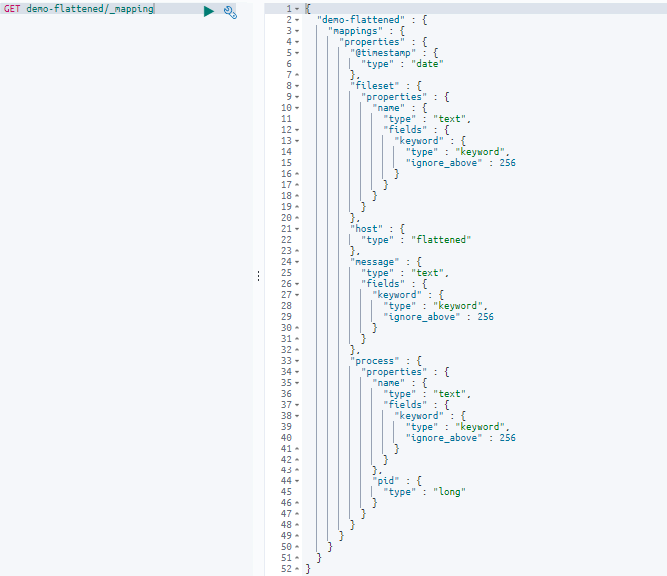
After indexing the sample document, let’s check the mapping of the index again by using in this request
GET demo-flattened/_mapping
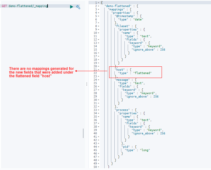
We can see here that Elasticsearch automatically mapped the fields to datatypes, except for the “host” field which remained the “flattened” type, as we previously configured it.
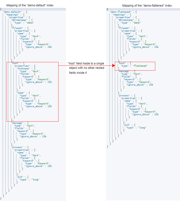
Now, let’s compare the mappings of the unflattened (demo-default) and flattened (demo-flattened) indexes.
Notice how our first non-flattened index created mappings for each individual field nested under the “host” object. In contrast, our latest flattened index shows a single mapping that throws all of the nested fields into one field, thereby reducing the amounts of fields in our index. And that’s precisely what we’re after here.
4.2 Adding New Fields Under a Flattened Object
We’ve seen how to create a flattened mapping for objects with a large number of nested fields. But what happens if additional nested fields need to flow into Elasticsearch after we’ve already mapped it?
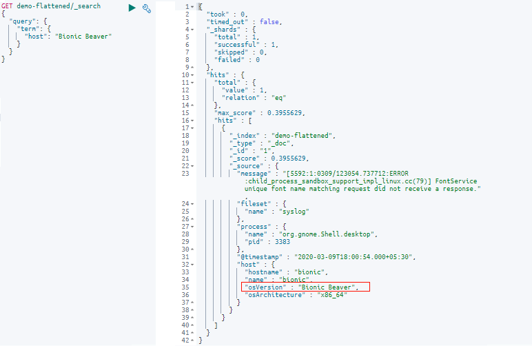
Let’s see how Elasticsearch reacts when we add more nested fields to the “host” object that has already been mapped to the flattened type.
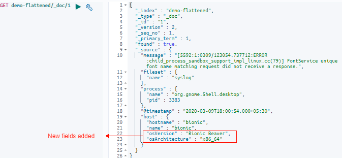
We’ll use Elasticsearch’s “update API” to POST an update to the “host” field and add two new sub-fields named “osVersion” and “osArchitecture” under “host”:
We can see here that the two fields were added successfully to the existing document.
Now let’s see what happens to the mapping of the “host” field:
GET demo-flattened/_mappings
Notice how our flattened mapping type for the “host” field has not been modified by Elasticsearch even though we’ve added two new fields. This is exactly the predictable behavior we want to have happened when indexing documents that can potentially generate a large number of fields. Since additional fields get mapped to the single flattened “host” field, no matter how many nested fields are added, the cluster state remains unchanged.
In this way, Elasticsearch helps us avoid the dreadful mapping explosions. However, as with many things in life, there’s a drawback to the flattened object approach and we’ll cover that next.
While it is possible to query the nested fields that get “flattened” inside a single field, there are certain limitations to be aware of. All field values in a flattened object are stored as keywords – and keyword fields don’t undergo any sort of text tokenization or analysis but are rather stored as-is.
The key capabilities that we lose by not having an “analyzed” field is the ability to use non-case sensitive queries so that you don’t have to enter an exact matching query and analyzed fields also enable Elasticsearch to factor the field into the search score.
Let’s take a look at some example queries to better understand these limitations so that we can choose the right mapping for different use cases.
5.1 Querying the top-level flattened field
There are a few nested fields under the field “host”. Let’s query the “host” field with a text query and see what happens:
Here in the results you can see we used the dot notation (host.osVersion) to refer to the inner field of “osVersion”.
5.3 Applying Match Queries
A match query returns the documents which match a text or phrase on one or more fields.
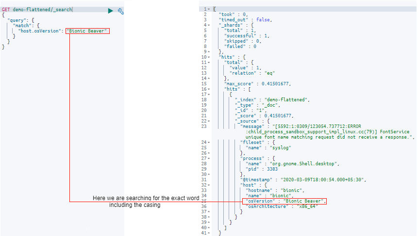
A match query can be applied to the flattened fields, but since the flattened field values are only stored as keywords, there are certain limitations for full-text search capabilities. This can be demonstrated best by performing three separate searches on the same field
5.3.1 Match Query Example 1
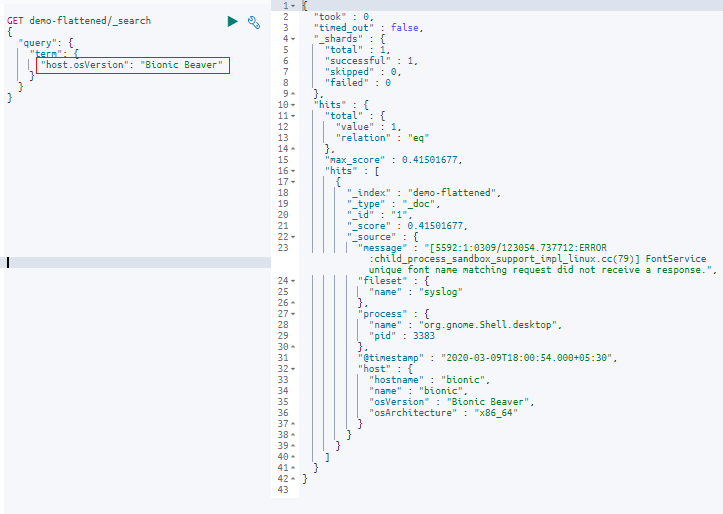
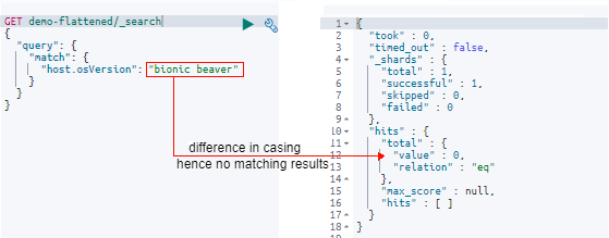
Let’s search the field “osVersion” inside the “host” field for the text “Bionic Beaver”. Here please notice the casing of the search text.
After passing in the search request, the query results will be as shown in the image:
Here you can see that the result contains the field “osVersion” with the value “Bionic Beaver” and is in the exact casing too.
5.3.2 Match Query Example 2
In the previous example, we saw the match query return the keyword with the exact same casing as that of the “osVersion” field. In this example, let’s see what happens when the search keyword differs from that in the field:
After passing the “match” query, we get no results. This is because the value stored in the “osVersion” field was exactly “Bionic Beaver” and since the field wasn’t analyzed by Elasticsearch as a result of using the flattening type, it will only return results matching the exact casing of the letters.
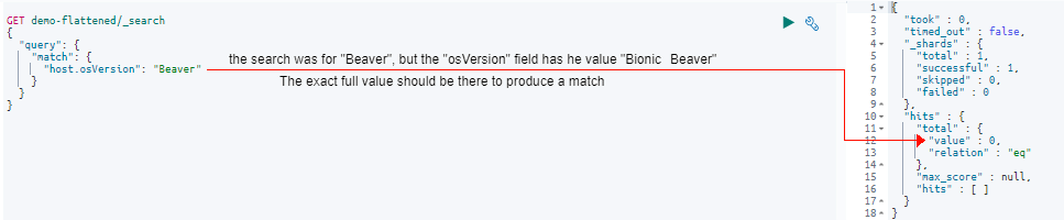
5.3.3 Match Query Example 3
Moving to our third example, let’s see the effect of querying just a part of the phrase of “Beaver” in the “osVersion” field:
In the response, you can see there are no matches. This is because our match query of “Beaver” doesn’t match the exact value of “Bionic Beaver” because the word “Bionic” is missing.
That was a lot of info, so let’s now summarise what we’ve learned with our example “match” queries on the host.osVersion field:
Match Query Text
Results
Reason
“Bionic Beaver”
Document returned with osVersion value as “Bionic Beaver”
Exact match of the match query text with that of the host.os Version’s value
“bionic beaver”
No documents returned
The casing of the match query text differs from that of host.osVersion (Bionic Beaver)
“Beaver”
No documents returned
The match query contains only a single token of “Beaver”. But the host.osVersion value is “Bionic Beaver” as a whole
6. Limitations
Whenever faced with the decision to flatten an object, here’s a few key limitations we need to consider when working with the Elasticsearch flattened datatype:
Supported query types are currently limited to the following:
term, terms, and terms_set
prefix
range
match and multi_match
query_string and simple_query_string
exists
Queries involving numeric calculations like querying a range of numbers, etc cannot be performed.
The results highlighting feature is not supported.
Even though the aggregations such as term aggregations are supported, the aggregations dealing with numerical data such as “histograms” or “date_histograms” are not supported.
7. Summary
In summary, we learned that Elasticsearch performance can quickly take a nosedive if we pump too many fields into an index. This is because the more fields we have the more memory required and Elasticsearch performance ends up taking a serious hit. This is especially true when dealing with limited resources or a high load.
The Elasticsearch flattened datatype is used to effectively reduce the number of fields contained in our index while still allowing us to query the flattened data.
However, this approach comes with its limitations, so choosing to use the “flattened” type should be reserved for cases that don’t require these capabilities.
Are you building and deploying software manually and would like to change that? Are you interested in learning about building a Jenkins pipeline and better understand CI/CD solutions and DevOps at the same time? In this first post, we will go over the fundamentals of how to design pipelines and how to implement them in Jenkins. Automation is the key to eliminating manual tasks and to reducing the number of errors while building, testing and deploying software. Let’s learn how Jenkins can help us achieve that with hands-on examples with the Jenkins parameters. By the end of this tutorial, you’ll have a broad understanding of how Jenkins works along with its Syntax and Pipeline examples.
What is a pipeline anyway?
Let’s start with a short analogy to a car manufacturing assembly line. I will oversimplify this to only three stages of a car’s production:
Bring the chassis
Mount the engine on the chassis
Place the body on the car
Even from this simple example, notice a few aspects:
These are a series of pipeline steps that need to be done in a particular order
The steps are connected: the output from the previous step is the input for the next step
In software development, a pipeline is a chain of processing components organized so that the output of one component is the input of the next component.
At the most basic level, a component is a command that does a particular task. The goal is to automate the entire process and to eliminate any human interaction. Repetitive tasks cost valuable time and often a machine can do repetitive tasks faster and more accurately than a human can do.
What is Jenkins?
Jenkins is an automation tool that automatically builds, tests, and deploys software from our version control repository all the way to our end users. A Jenkins pipeline is a sequence of automated stages and steps to enable us to accelerate the development process – ultimately achieving Continuous Delivery (CD). Jenkins helps to automatically build, test, and deploy software without any human interaction – but we will get into that a bit later.
If you don’t already have Jenkins installed, make sure that you check this installation guide to get you started.
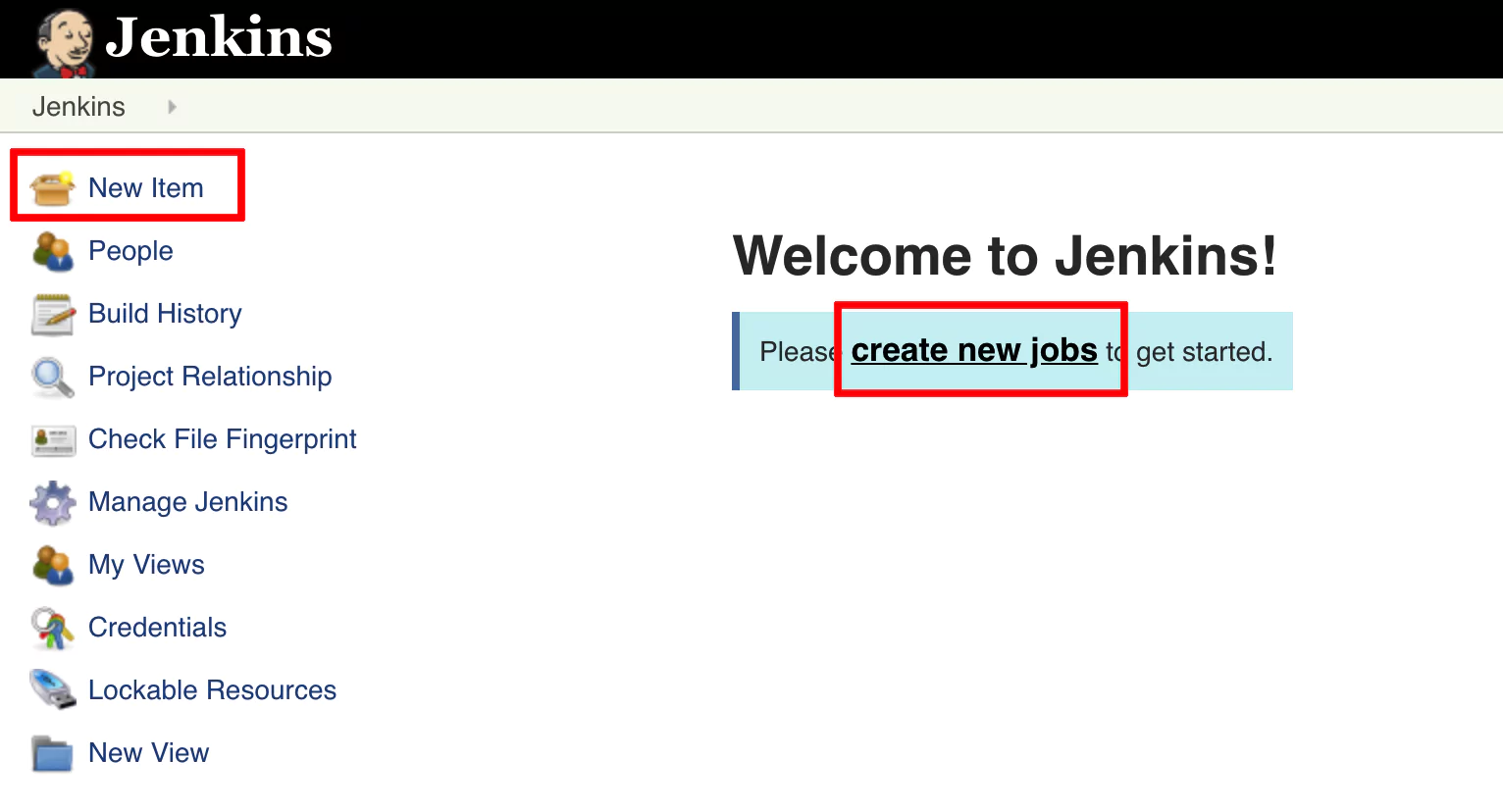
Create a Jenkins Pipeline Job
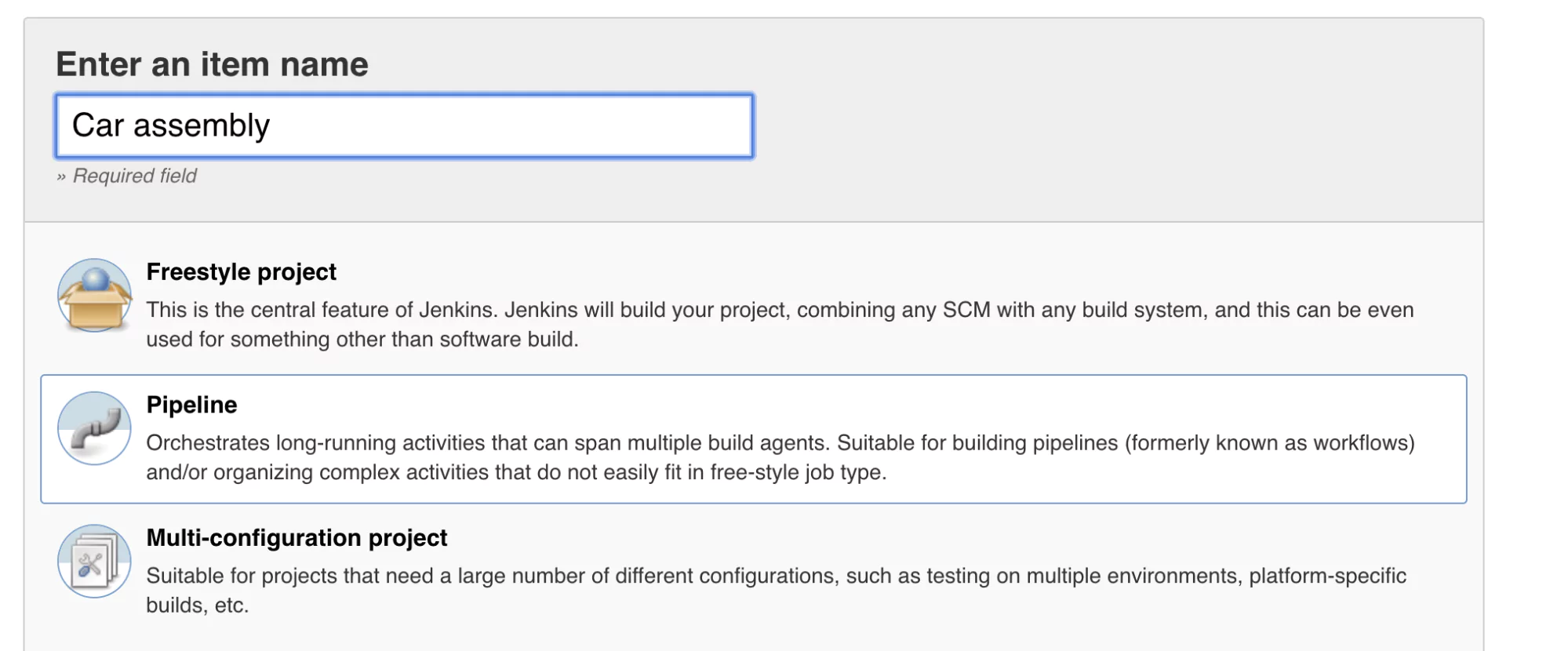
Let’s go ahead and create a new job in Jenkins. A job is a task or a set of tasks that run in a particular order. We want Jenkins to automatically execute the task or tasks and to record the result. It is something we assign Jenkins to do on our behalf.
Click on Create new jobs if you see the text link, or from the left panel, click on New Item (an Item is a job).
Name your job Car assembly and select the Pipeline type. Click ok.
Configure Pipeline Job
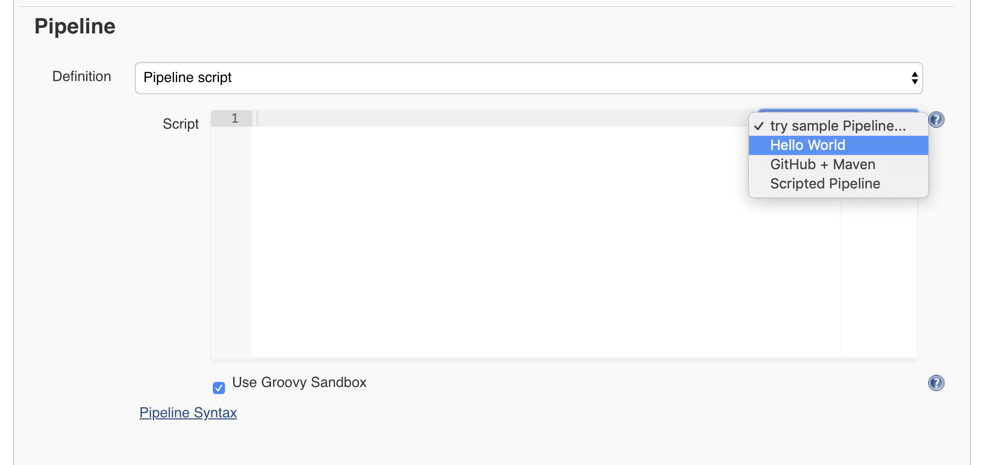
Now you will get to the job configuration page where we’ll configure a pipeline using the Jenkins syntax. At first, this may look scary and long, but don’t worry. I will take you through the process of building Jenkins pipeline step by step with every parameter provided and explained. Scroll to the lower part of the page until you reach a part called Pipeline. This is where we can start defining our Jenkins pipeline. We will start with a quick example. On the right side of the editor, you will find a select box. From there, choose Hello World.
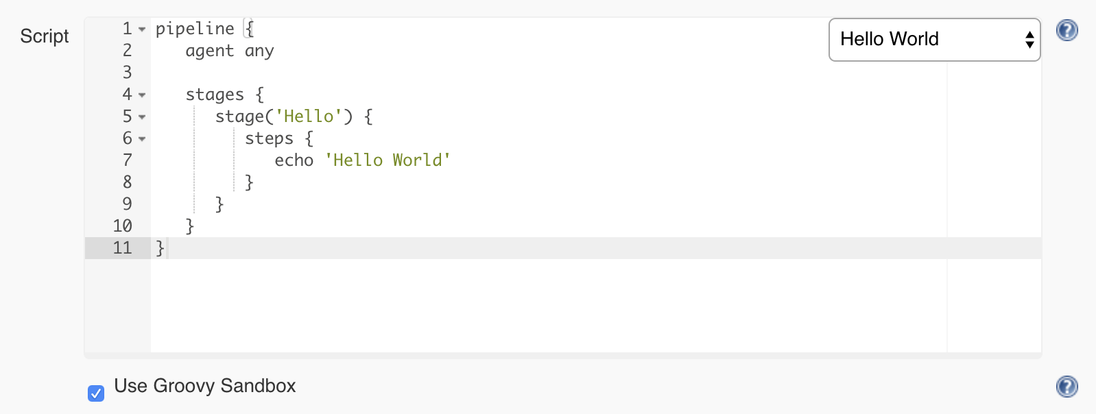
You will notice that some code was generated for you. This is a straightforward pipeline that only has one step and displays a message using the command echo ‘Hello World’.
Click on Save and return to the main job page.
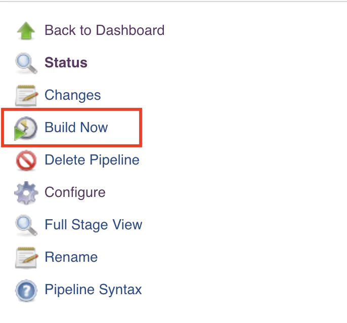
Build The Jenkins Pipeline
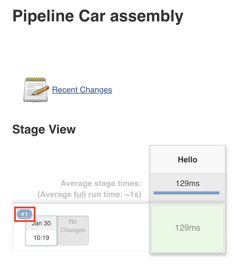
From the left-side menu, click on Build Now.
This will start running the job, which will read the configuration and begin executing the steps configured in the pipeline. Once the execution is done, you should see something similar to this layout:
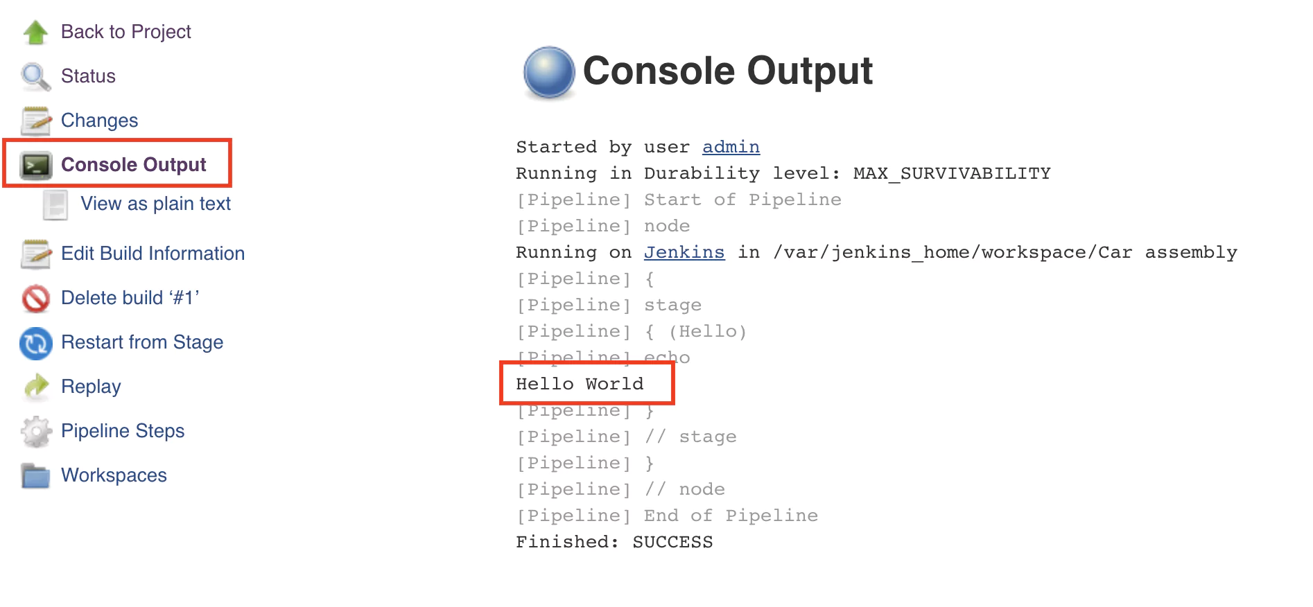
A green-colored stage will indicate that the execution was successful and no errors where encountered. To view the console output, click on the number of the build (in this case #1). After this, click on the Console output button, and the output will be displayed.
Notice the text Hello world that was displayed after executing the command echo ‘Hello World’.
Congratulations! You have just configured and executed your first pipeline in Jenkins.
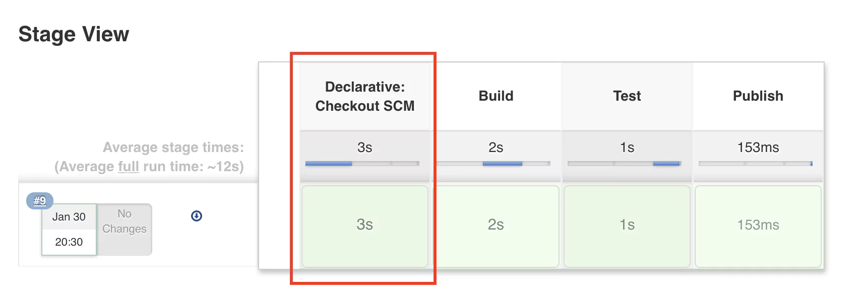
A Basic Pipeline Build Process
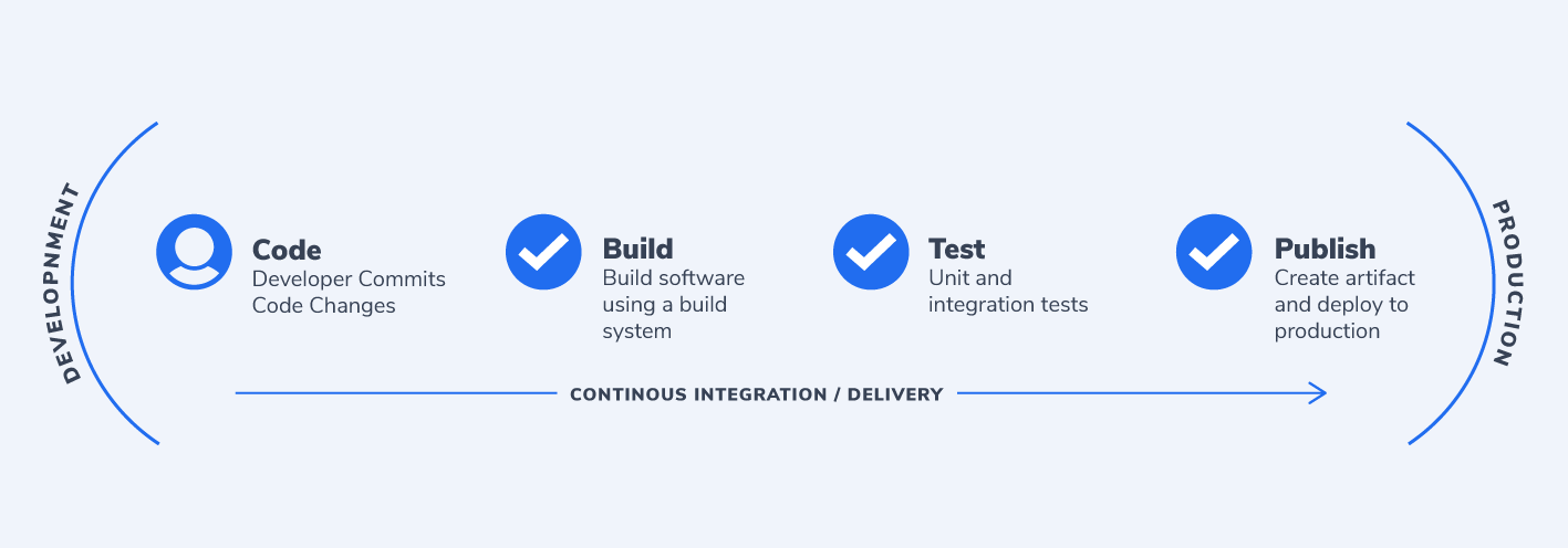
When building software, we usually go through several stages. Most commonly, they are:
Build – this is the main step and does the automation work required
Test – ensures that the build step was successful and that the output is as expected
Publish – if the test stage is successful, this saves the output of the build job for later use
We will create a simple car assembly pipeline but only using folders, files, and text. So we want to do the following in each stage:
Build
create a build folder
create a car.txt file inside the build folder
add the words “chassis”, “engine” and “body” to the car.txt file
Test
check that the car.txt file exists in the build folder
words “chassis”, “engine” and “body” are present in the car.txt file
Publish
save the content of the build folder as a zip file
The Jenkins Build Stage
Note: the following steps require that Jenkins is running on a Unix-like system. Alternatively, the Windows system running Jenkins should have some Unix utilities installed.
Let’s go back to the Car assembly job configuration page and rename the step that we have from Hello to Build. Next, using the pipeline step sh, we can execute a given shell command. So the Jenkins pipeline will look like this:
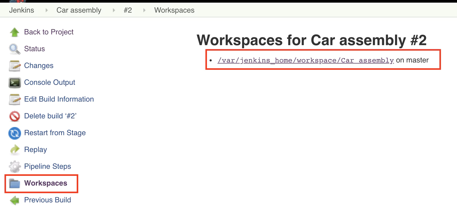
Let’s save and execute the pipeline. Hopefully, the pipeline is successful again, but how do we know if the car.txt file was created? Do inspect the output, click on the job number and on the next page from the left menu select Workspaces.
Click on the folder path displayed and you should soon see the build folder and its contents.
The Jenkins Test Stage
In the previous step, we manually checked that the folder and the file were created. As we want to automate the process, it makes sense to write a test that will check if the file was created and has the expected contents.
Let’s create a test stage and use the following commands to write the test:
the test command combined with the -f flag allows us to test if a file exists
the grep command will enable us to search the content of a file for a specific string
So the pipeline will look like this:
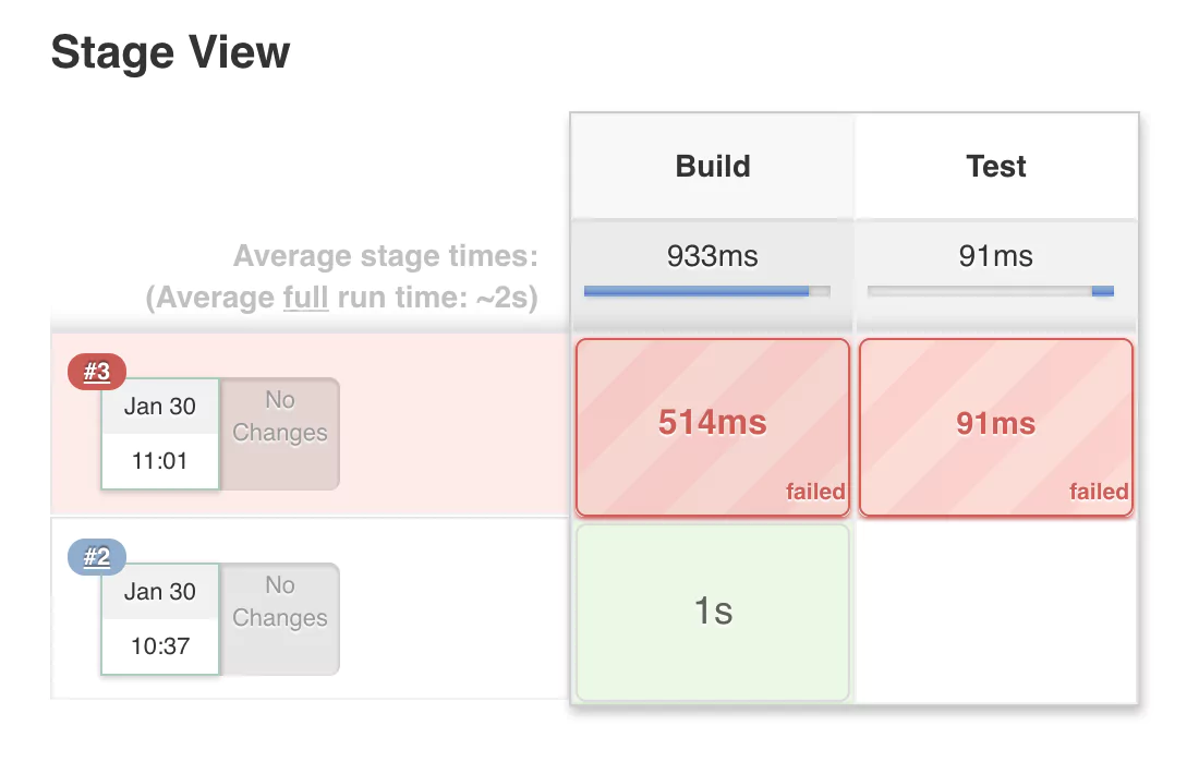
Why did the Jenkins pipeline fail?
If you save the previous configuration and run the pipeline again, you will notice that it will fail, indicated by a red color.
The most common reasons for a pipeline to fail is because:
The pipeline configuration is incorrect. This first problem is most likely due to a syntax issue or because we’ve used a term that was not understood by Jenkins.
One of the build step commands returns a non-zero exit code. This second problem is more common. Each command after executing is expected to return an exit code. This tells Jenkins if the command was successful or not. If the exit code is 0, it means the command was successful. If the exit code is not 0, the command encountered an error.
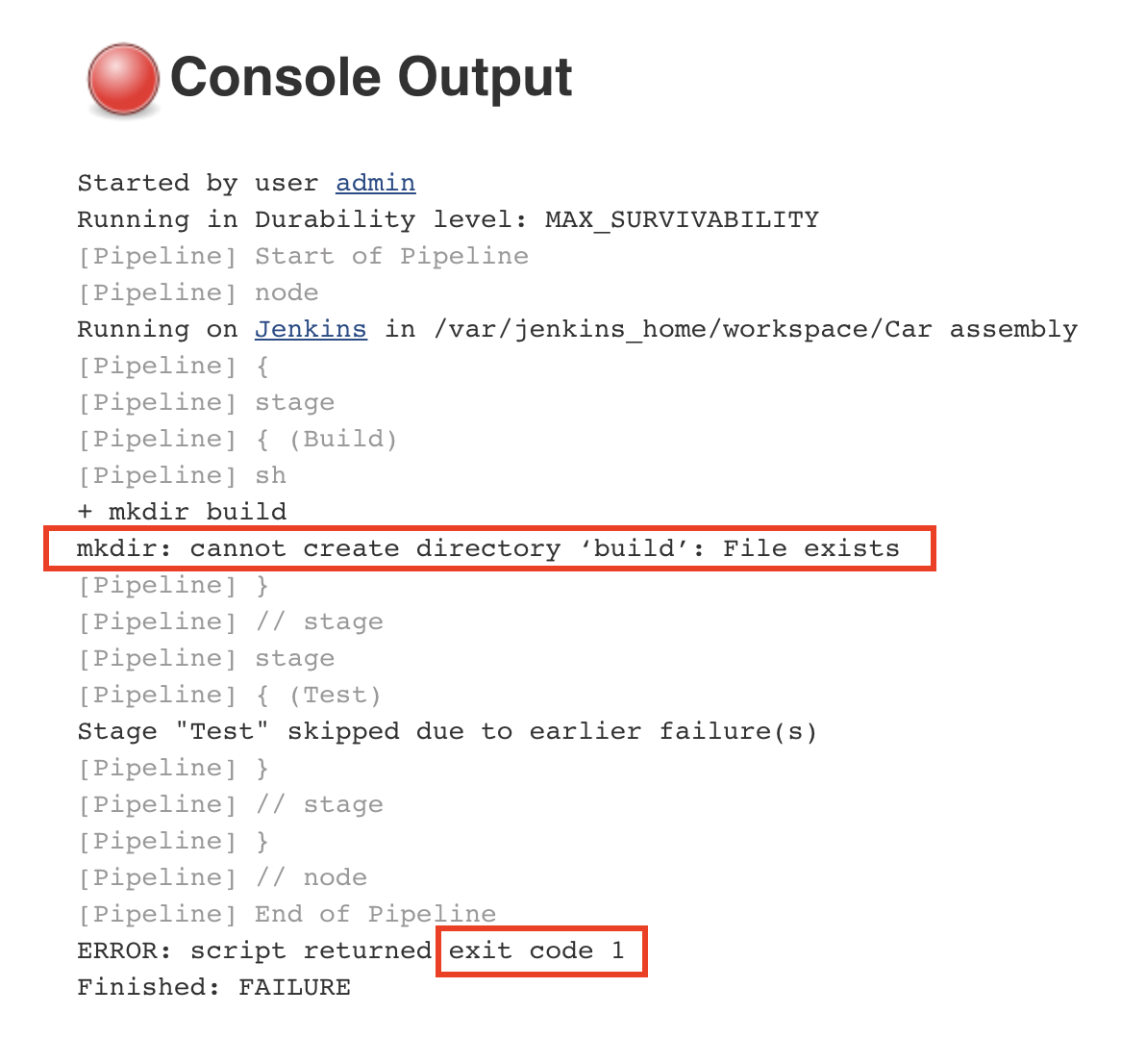
We want to stop the execution of the pipeline as soon as an error has been detected. This is to prevent future steps from running and propagating the error to the next stages. If we inspect the console output for the pipeline that has failed, we will identify the following error:
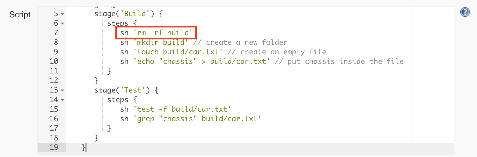
The error tells us that the command could not create a new build folder as one already exists. This happens because the previous execution of the pipeline already created a folder named ‘build’. Every Jenkins job has a workspace folder allocated on the disk for any files that are needed or generated for and during the job execution. One simple solution is to remove any existing build folder before creating a new one. We will use the rm command for this.
This will make the pipeline work again and also go through the test step.
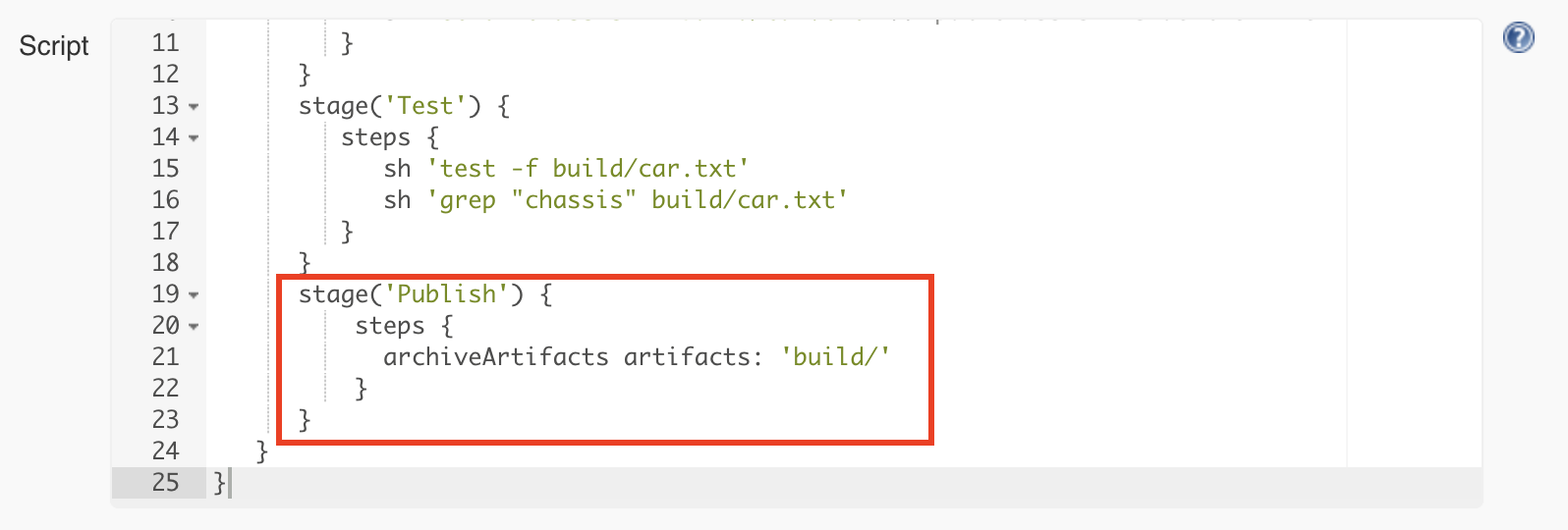
The Jenkins Publishing Stage
If the tests are successful, we consider this a build that we want to keep for later use. As you remember, we remove the build folder when starting rerunning the pipeline, so it does not make sense to keep anything in the workspace of the job. The job workspace is only for temporary purposes during the execution of the pipeline. Jenkins provides a way to save the build result using a build step called archiveArtifacts.
So what is an artifact? In archaeology, an artifact is something made or given shape by humans. Or in other words, it’s an object. Within our context, the artifact is the build folder containing the car.txt file.
We will add the final stage responsible for publishing and configuring the archiveArtifacts step to publish only the contents of the build folder:
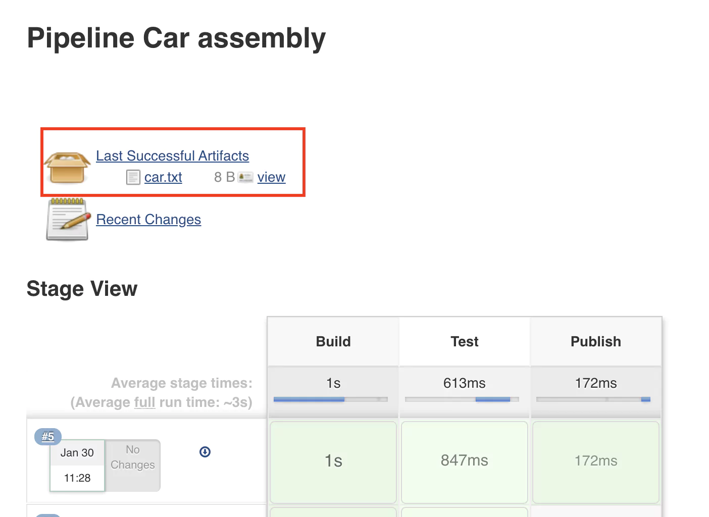
After rerunning the pipeline, the job page will display the latest successful artifact. Refresh the page once or twice if it does not show up.
(17-last-artifact.png)
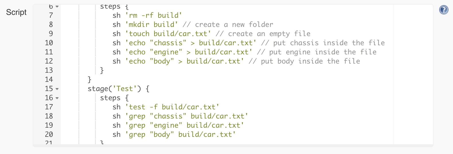
Complete & Test the Pipeline
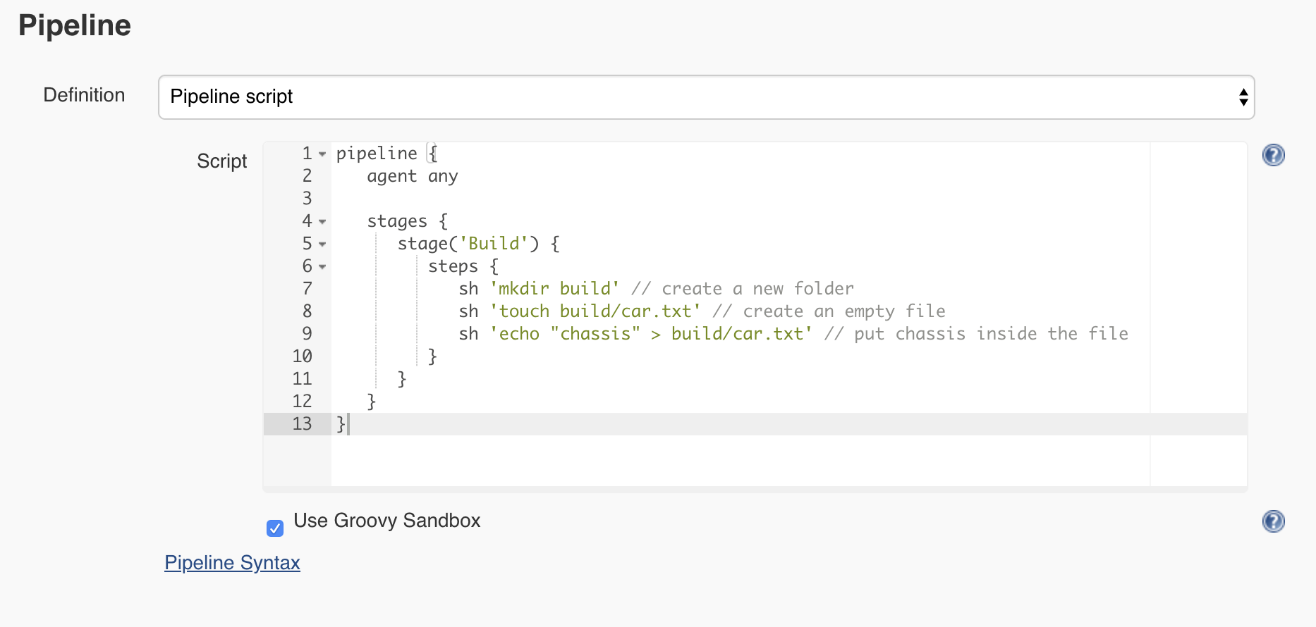
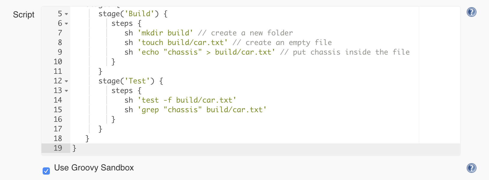
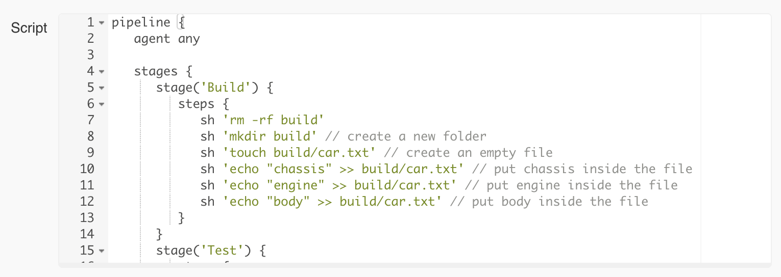
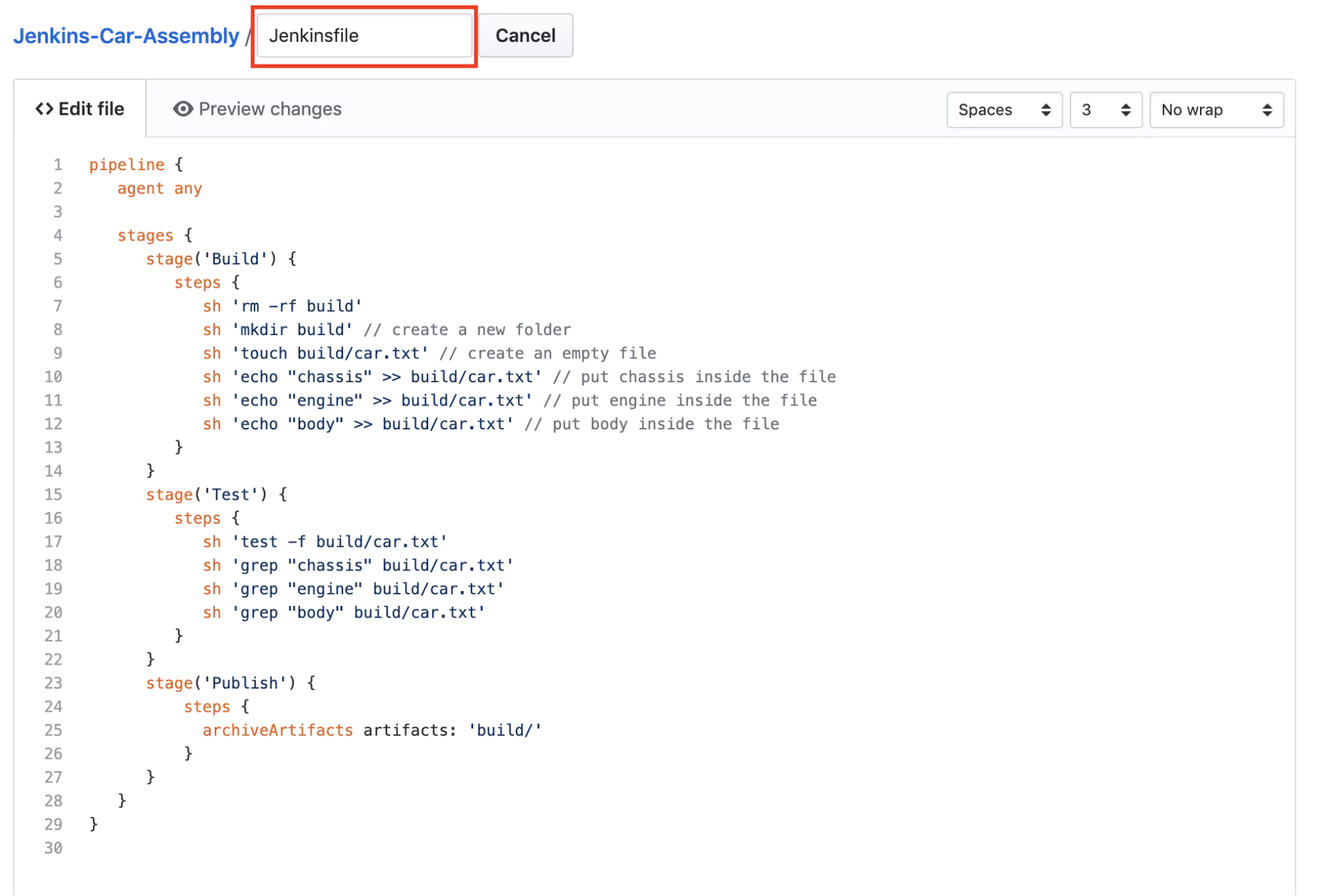
Let’s continue adding the other parts of the car: the engine and the body. For this, we will adapt both the build and the test stage as follows:
pipeline {
   agent any

   stages {
      stage('Build') {
         steps {
            sh 'rm -rf build'
            sh 'mkdir build' // create a new folder
            sh 'touch build/car.txt' // create an empty file
            sh 'echo "chassis" > build/car.txt' // add chassis
            sh 'echo "engine" > build/car.txt' // add engine
            sh 'echo "body" > build/car.txt' // body
         }
      }
      stage('Test') {
          steps {
              sh 'test -f build/car.txt'
              sh 'grep "chassis" build/car.txt'
              sh 'grep "engine" build/car.txt'
              sh 'grep "body" build/car.txt'
          }
      }
   }
}
Saving and rerunning the pipeline with this configuration will lead to an error in the test phase.
The reason for the error is that the car.txt file now only contains the word “body”. Good that we tested it! The > (greater than) operator will replace the entire content of the file, and we don’t want that. So we’ll use the >> operator just to append text to the file.
pipeline {
   agent any

   stages {
      stage('Build') {
         steps {
            sh 'rm -rf build'
            sh 'mkdir build'
            sh 'touch build/car.txt'
            sh 'echo "chassis" >> build/car.txt'
            sh 'echo "engine" >> build/car.txt'
            sh 'echo "body" >> build/car.txt'
         }
      }
      stage('Test') {
          steps {
              sh 'test -f build/car.txt'
              sh 'grep "chassis" build/car.txt'
              sh 'grep "engine" build/car.txt'
              sh 'grep "body" build/car.txt'
          }
      }
   }
}
Now the pipeline is successful again, and we’re confident that our artifact (i.e. file) has the right content.
Pipeline as Code
If you remember, at the beginning of the tutorial, you were asked to select the type of job you want to create. Historically, many jobs in Jenkins were and still are configured manually, with different checkboxes, text fields, and so on. Here we did something different. We called this approach Pipeline as Code. While it was not apparent, we’ve used a Domain Specific Language (DSL), which has its foundation in the Groovy scripting language. So this is the code that defines the pipeline.
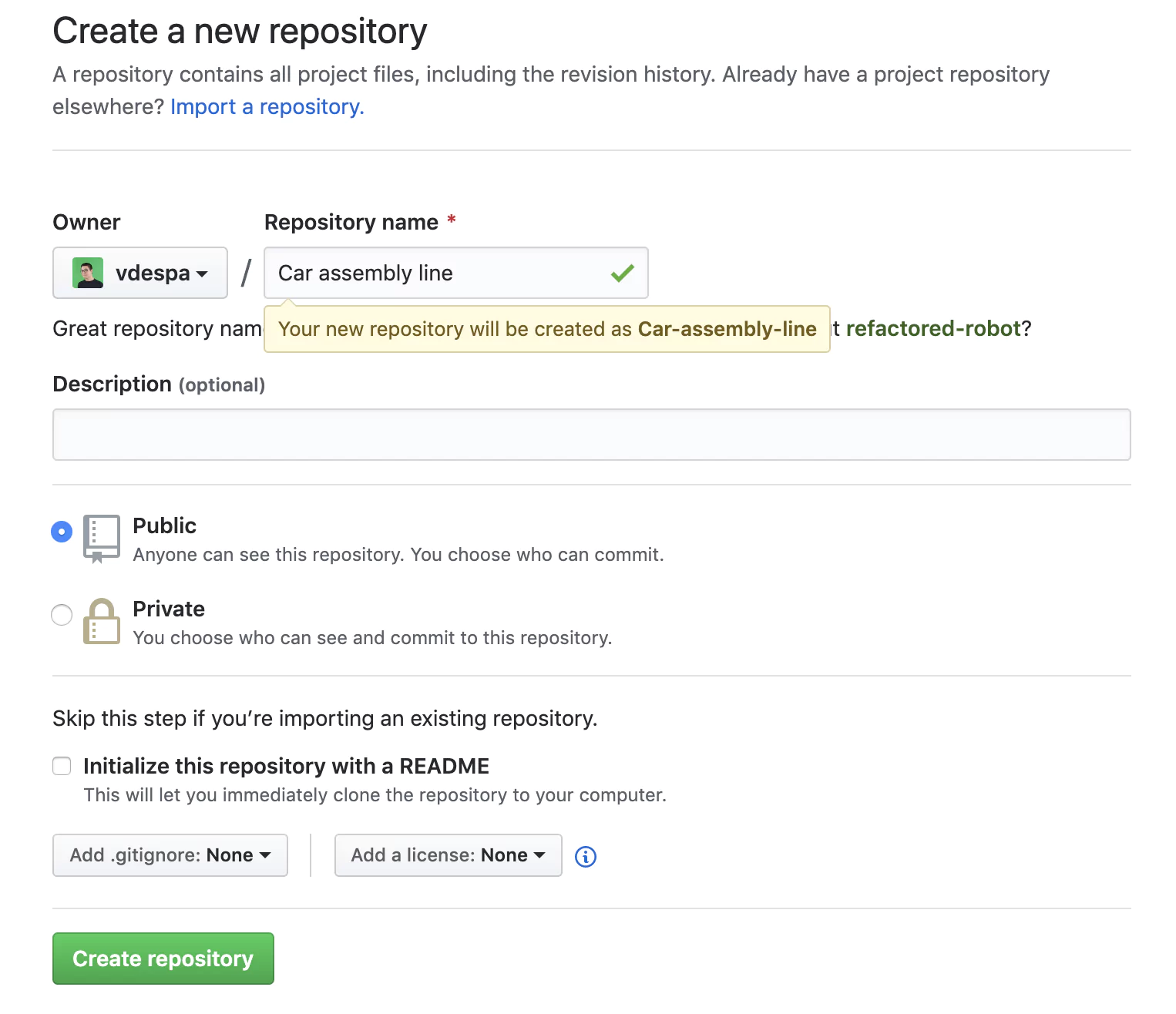
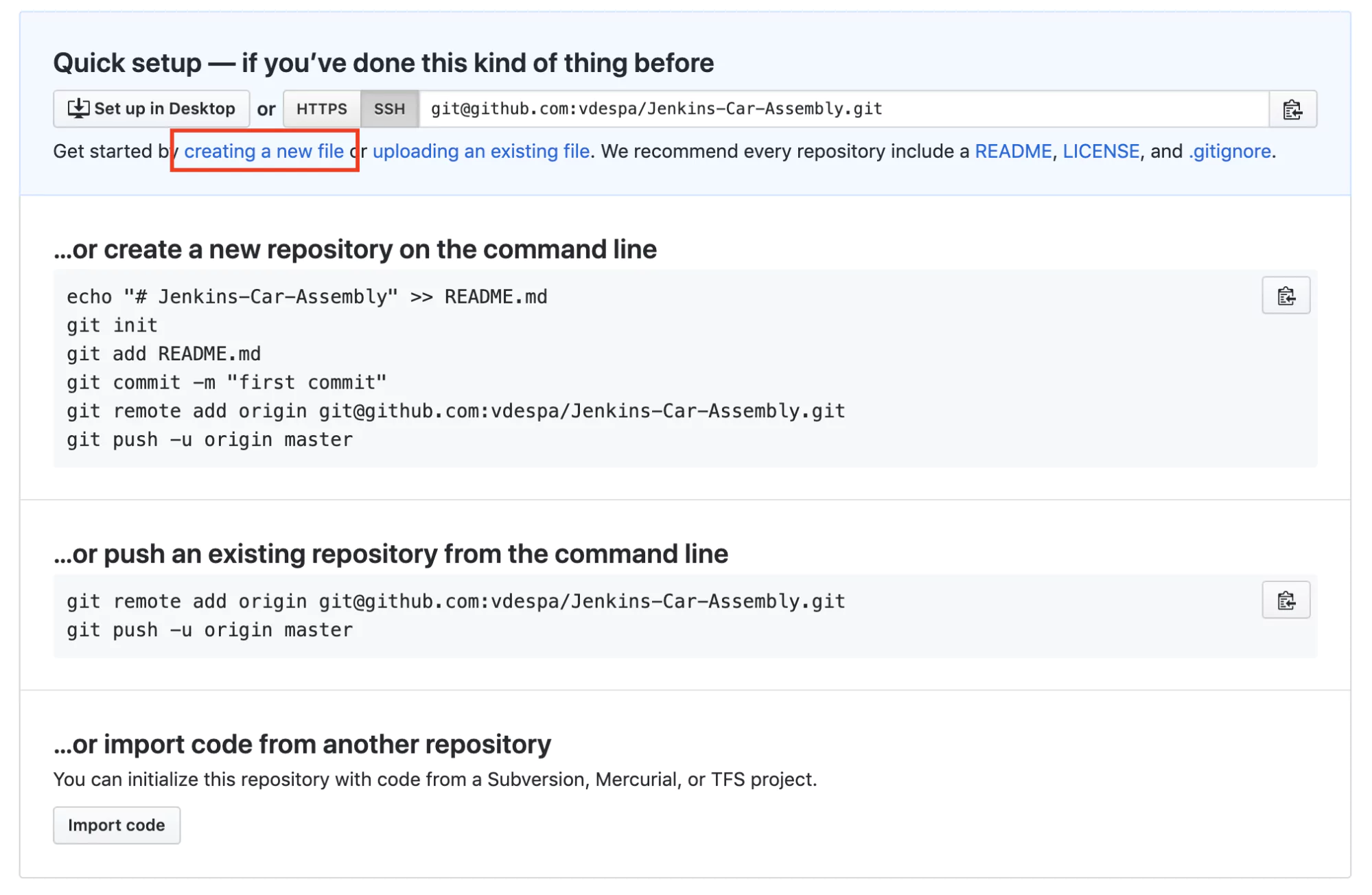
As you can observe, even for a relatively simple scenario, the pipeline is starting to grow in size and become harder to manage. Also, configuring the pipeline directly in Jenkins is cumbersome without a proper text editor. Moreover, any work colleagues with a Jenkins account can modify the pipeline, and we wouldn’t know what changed and why. There must be a better way! And there is. To fix this, we will create a new Git repository on Github.
To make things simpler, you can use this public repository under my profile called Jenkins-Car-Assembly.
Jenkinsfile from a Version Control System
The next step is to create a new file called Jenkinsfile in your Github repository with the contents of the pipeline from Jenkins.
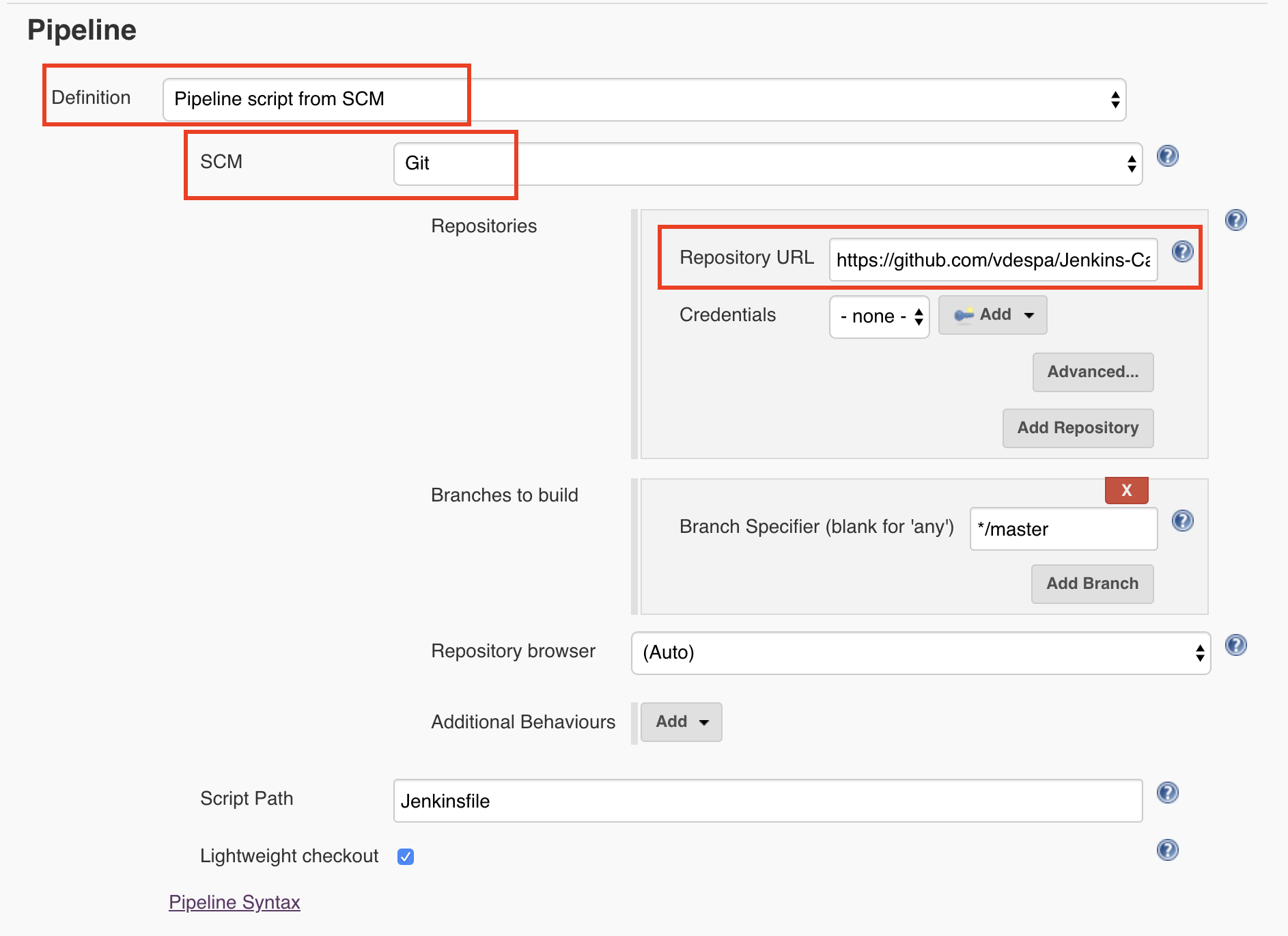
Read Pipeline from Git
Finally, we need to tell Jenkins to read the pipeline configuration from Git. I have selected the Definition as Pipeline Script from SCM which in our case, refers to Github. By the way, SCM stands for Source code management.
Saving and rerunning the pipeline leads to a very similar result.
So what happened? Now we use Git to store the pipeline configuration in a file called Jenkinsfile. This allows us to use any text editing software to change the pipeline but now we can also keep track of any changes that happen to the configuration. In case something doesn’t work after making a Jenkins configuration change, we can quickly revert to the previous version.
Typically, the Jenkinsfile will be stored in the same Git repository as the project we are trying to build, test, and release. As a best practice, we always store code in an SCM system. Our pipeline belongs there as well, and only then can we really say that we have a ‘pipeline as code’.
Conclusion
I hope that this quick introduction to Jenkins and pipelines has helped you understand what a pipeline is, what are the most typical stages, and how Jenkins can help automate the build and test process and ultimately deliver more value to your users faster.
For your reference, you can find the Github repository referenced in this tutorial here:
Elasticsearch is a popular distributed search and analytics engine designed to handle large volumes of data for fast, real-time searches. Elasticsearch’s capabilities make it useful in many essential cases like log analysis. Its users can create their own analytics queries, or use existing platforms like Coralogix to streamline analyzing data stored in an index.
We’ve created a hands-on tutorial to help you take advantage of the most important queries that Elasticsearch has to offer. In this guide, you’ll learn 42 popular Elasticsearch query examples with detailed explanations. Each query covered here will fall into 2 types:
Structured Queries: queries that are used to retrieve structured data such as dates, numbers, pin codes, etc.
Full-text Queries: queries that are used to query plain text.
Note: For this article and the related operations, we’re using Elasticsearch and Kibana version 8.9.0.
Here’s primary query examples that will be covered in the guide:
Elasticsearch queries are put into a search engine to find specific documents from an index, or from multiple indices. Elasticsearch was designed as a distributed, RESTful search and analytics engine, making it useful for full-text searching, real-time analytics, and data visualization. It is efficient at searching large volumes of data.
Elasticsearch was designed as a powerful search interface. The various available queries are flexible and allow users to search and aggregate data to find the most useful information.
Elasticsearch query types
Lucene Query Syntax
The Apache Lucene search library is an open-source, high-performance, full-text search library developed in Java. This library is the foundation upon which Elasticsearch was built, so is integral to how Elasticsearch functions.
The Lucene query syntax allows users to construct complex queries for retrieving documents from indices in Elasticsearch. These include field-based searches for terms within text fields, boolean operations between search terms, wildcard queries, and proximity searches. These extra features are used within Elasticsearch’s Query syntax, and you will see these present in the examples shown in this article.
Query Syntax
The Elasticsearch query syntax, shown in the example set below, is based on JSON notation. These objects define the criteria and conditions allowing for specific documents to be retrieved from the index. Users define query types within the JSON to define the search scenario.
Examples of query types that will be covered in examples are match queries for full-text searches, term queries for exact matches, and bool queries for combining conditions. Developers can also customize search behaviors by leveraging scripting using Painless.
Painless is a lightweight scripting language introduced by Elasticsearch to provide scripting capabilities for various operations within Elasticsearch. This scripting operates within the Elasticsearch environment and interacts with the underlying Lucene index.
Painless is used for customizing queries, aggregations, and data transformations during search and indexing processes.
Setup The Demo Index
If you are unfamiliar with Elasticsearch’s basic usage and setup, check out this introduction to Elasticsearch before proceeding. For this tutorial, let’s start with creating a new index with some sample data so that you can follow along for each search example. Create an index named “employees”
PUT employees
Define a mapping (schema) for one of the fields (date_of_birth) that will be contained in the ingested document (the following step after this). Note that any fields not defined in the mapping but that are added to the index will be given default types in the mapping.
Now that we have an index with documents and a mapping specified, we’re ready to get started with the example searches.
1. Match Query
The “match” query is one of the most basic and commonly used queries in Elasticsearch and functions as a full-text query. We can use this query to search for text, number, or boolean values.
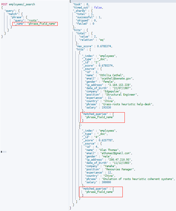
Let us search for the word “heuristic” in the ” phrase ” field in the documents we ingested earlier.
This returns the same document as before because by default, Elasticsearch treats each word in the search query with an OR operator. In our case, the query will match any document that contains “heuristic” OR “roots” OR “help.”
Changing The Operator Parameter The default behavior of the OR operator being applied to multi-word searches can be changed using the “operator” parameter passed along with the “match” query. We can specify the operator parameter with “OR” or “AND” values. Let’s see what happens when we provide the operator parameter “AND” in the same query we performed earlier.
Now the results will return only one document (document id=2) since that is the only document containing all three search keywords in the “phrase” field.
minimum_should_match
Taking things a bit further, we can set a threshold for a minimum amount of matching words that the document must contain. For example, if we set this parameter to 1, the query will check for any documents with a minimum of 1 matching word. Now, if we set the “minium_should_match” parameter to 3, then all three words must appear in the document to be classified as a match.
In our case, the following query would return only 1 document (with id=2) as that is the only one matching our criteria
So far we’ve been dealing with matches on a single field – that is we searched for the keywords inside a single field named “phrase.” But what if we needed to search keywords across multiple fields in a document? This is where the multi-match query comes into play. Let’s try an example search for the keyword “research help” in the “position” and “phrase” fields contained in the documents.
Match_phrase is another commonly used query which, like its name indicates, matches phrases in a field. If we need to search for the phrase “roots heuristic coherent” in the “phrase” field in the employee index, we can use the “match_phrase” query:
This will return the documents with the exact phrase “roots heuristic coherent”, including the order of the words. In our case, we have only one result matching the above criteria, as shown in the below response
A useful feature we can make use of in the match_phrase query is the “slop” parameter which allows us to create more flexible searches. Suppose we searched for “roots coherent” with the match_phrase query. We wouldn’t receive any documents returned from the employee index. This is because for match_phrase to match, the terms need to be in the exact order. Now, let’s use the slop parameter and see what happens:
With slop=1, the query is indicating that it is okay to move one word for a match, and therefore we’ll receive the following response. In the below response, you can see that the “roots coherent” matched the “roots heuristic coherent” document. This is because the slop parameter allows skipping 1 term.
The match_phrase_prefix query is similar to the match_phrase query, but here the last term of the search keyword is considered as a prefix and is used to match any term starting with that prefix term. First, let’s insert a document into our index to better understand the match_phrase_prefix query:
In the results below, we can see that the documents with coherent and complete matched the query. We can also use the slop parameter in the “match_phrase” query.
Note: “match_phrase_query” tries to match 50 expansions (by default) of the last provided keyword (co in our example). This can be increased or decreased by specifying the “max_expansions” parameter. Due to this prefix property and the easy to set up property of the match_phrase_prefix query, it is often used for autocomplete functionality. Now let’s delete the document we just added with id=5:
DELETE employees/_doc/5
2. Term Level Queries
Term-level queries are used to query structured data, which would usually be the exact values.
2.1. Term Query/Terms Query
This is the simplest of the term-level queries. This query searches for the exact match of the search keyword against the field in the documents. For example, if we search for the word “Male” using the term query against the field “gender”, it will search exactly as the word is, even with the casing. This can be demonstrated by the below two queries:
In the above case, the only difference between the two queries is that of the casing of the search keyword. Case 1 had all lowercase, which was matched because that is how it was saved against the field. But for Case 2, the search didn’t get any result, because there was no such token against the field “gender” with a capitalized “F”
We can also pass multiple terms to be searched on the same field, by using the terms query. Let us search for “female” and “male” in the gender field. For that, we can use the terms query as below:
Sometimes it happens that there is no indexed value for a field, or the field does not exist in the document. In such cases, it helps in identifying such documents and analyzing the impact. For example, let us index a document like the below to the “employees” index
The above query will list all the documents which have the field “company”. Perhaps a more useful solution would be to list all the documents without the “company” field. This can also be achieved by using the exist query as below
The bool query is explained in detail in the following sections. Let us delete the now inserted document from the index, for the cause of convenience and uniformity by typing in the below request
DELETE employees/_doc/5
2.3 Range Queries
Another most commonly used query in the Elasticsearch world is the range query. The range query allows us to get the documents that contain the terms within the specified range. Range query is a term level query (means using to query structured data) and can be used against numerical fields, date fields, etc.
Range query on numeric fields
For example, in the data set, we have created, if we need to filter out the people who have experience level between 5 to 10 years, we can apply the following range query for the same:
Greater than or equal to. gte: 5 , means greater than or equal to 5, which includes 5
gt
Greater than. gt: 5 , means greater than 5, which does not include 5
lte
Less than or equal to. lte: 5 , means less than or equal to 5, which includes 5
lt
Less than. gt: 5 , means less than 5, which does not include 5
Range query on date fields
Similarly, range queries can be applied to the date fields as well. If we need to find out those who were born after 1986, we can fire a query like the one given below:
This will fetch us the documents which have the date_of_birth fields only after the year 1986.
2.4 Ids Queries
The ids query is a relatively less used query but is one of the most useful ones and hence qualifies to be in this list. There are occasions when we need to retrieve documents based on their IDs. This can be achieved using a single get request as below:
GET indexname/typename/documentId
This can be a good solution if there is only one document to be fetched by an ID, but what if we have many more?
That is where the ids query comes in very handy. With the ids query, we can do this in a single request. In the below example, we are fetching documents with ids 1 and 4 from the employee index with a single request.
The prefix query is used to fetch documents that contain the given search string as the prefix in the specified field. Suppose we need to fetch all documents which contain “al” as the prefix in the field “name”, then we can use the prefix query as below:
Since the prefix query is a term query, it will pass the search string as it is. That is, searching for “al” and “Al” is different. If in the above example, we search for “Al”, we will get 0 results as there is no token starting with “Al” in the inverted index of the field “name”. But if we query on the field “name.keyword”, with “Al” we will get the above result and in this case, querying for “al” will result in zero hits.
2.6 Wildcard Queries
Will fetch the documents that have terms that match the given wildcard pattern. For example, let us search for “c*a” using the wildcard query on the field “country” like below:
The above query will fetch all the documents with the “country” name starting with “c” and ending with “a” (eg: China, Canada, Cambodia, etc).
Here the * operator can match zero or more characters.
Note that wildcard queries and regexp queries described below can become expensive, especially when the ‘*’ symbol is used at the beginning of the search pattern. These queries need to be enabled for the index using the “search.allow_expensive_queries” parameter.
2.7 Regexp
This is similar to the “wildcard” query we saw above but will accept regular expressions as input and fetch documents matching those.
The above query will get us the documents matching the words that match the regular expression res[a-z]*
2.8 Fuzzy
The Fuzzy query can be used to return documents containing terms similar to that of the search term. This is especially good when dealing with spelling mistakes. We can get results even if we search for “Chnia” instead of “China”, using the fuzzy query. Let us have a look at an example:
Here fuzziness is the maximum edit distance allowed for matching. The parameters like “max_expansions” etc., which we saw in the “match_phrase” query can also be used. More documentation on the same can be found here.
Fuzzy queries can also come in with the “match” query types. The following example shows the fuzziness being used in a multi_match query
The above query will return the documents matching either “heuristic” or “research” despite the spelling mistakes in the query.
3. Boosting
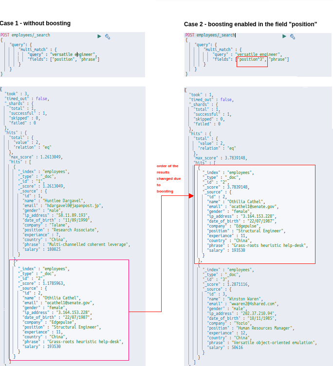
While querying, it is often helpful to get the more favored results first. The simplest way of doing this is called boosting in Elasticsearch. And this comes in handy when we query multiple fields. For example, consider the following query:
This will return the response with the documents matching the “position” field to be in the top rather than with that of the field “phrase”.
4. Sorting
4.1 Default Sorting
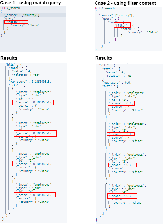
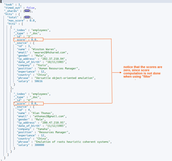
When there is no sort parameter specified in the search request, Elasticsearch returns the document based on the descending values of the “_score” field. This “_score” is computed by how well the query has matched using the default scoring methodologies of Elasticsearch. In all the examples we have discussed above you can see the same behavior in the results. It is only when we use the “filter” context that there is no scoring computed, so as to make the return of the results faster.
4.2 How to Sort by a Field
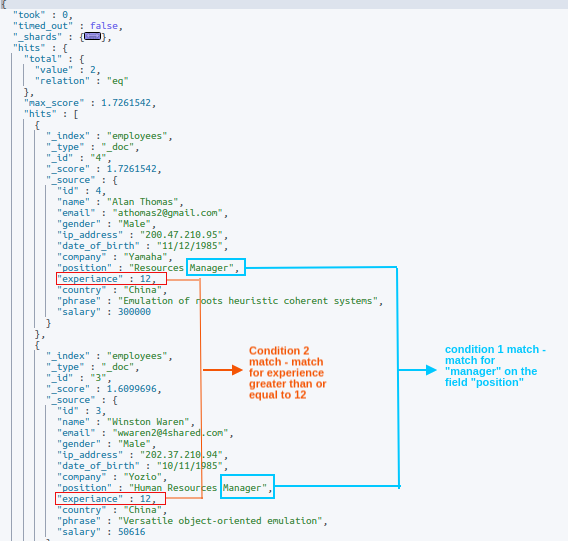
Elasticsearch gives us the option to sort on the basis of a field. Say, let us need to sort the employees based on their descending order of experience. We can use the below query with the sort option enabled to achieve that:
As you can see from the above response, the results are ordered based on the descending values of the employee experience. Also, there are two employees, with the same experience level as 12.
4.3 How to Sort by Multiple Fields
In the above example, we saw that there are two employees with the same experience level of 12, but we need to sort again based on the descending order of the salary. We can provide multiple fields for sorting too, as shown in the query demonstrated below:
In the above results, you can see that within the employees having same experience levels, the one with the highest salary was promoted early in the order (Alan and Winston had same experience levels, but unlike the previous search results, here Alan was promoted as he had higher salary).
Note: If we change the order of sort parameters in the sorted array, that is if we keep the “salary” parameter first and then the “experience” parameter, then the search results would also change. The results will first be sorted on the basis of the salary parameter and then the experience parameter will be considered, without impacting the salary-based sorting.
Let us invert the order of sort of the above query, that is “salary” is kept first and the “experience” as shown below:
You can see that the candidate with experience value 12 came below the candidate with experience value 7, as the latter had more salary than the former.
5. Compound Queries
So far, in the tutorial, we have seen that we fired single queries, like finding a text match or finding the age ranges, etc. But more often in the real world, we need multiple conditions to be checked and documents to be returned based on that. Also, we might need to modify the relevance or score parameter of the queries or to change the behavior of the individual queries, etc. Compound queries are the queries that help us to achieve the above scenarios. In this section, let us have a look into a few of the most helpful compound queries.
5.1. The Bool Query
Bool query provides a way to combine multiple queries in a boolean manner. That is for example if we want to retrieve all the documents with the keyword “researcher” in the field “position” and those who have more than 12 years of experience we need to use the combination of the match query and that of the range query. This kind of query can be formulated using the bool query. The bool query has mainly 4 types of occurrences defined:
must
The conditions or queries in this must occur in the documents to consider them a match. Also, this contributes to the score value. For example, if we keep query A and query B in the must section, each document in the result would satisfy both the queries, i.e. query A AND query B
should
The conditions/queries should match. Result = query A OR query B
filter
Conditions are the same as the must clause, but no score will be calculated.
must_not
The conditions/queries specified must not occur in the documents. Scoring is ignored and kept as 0 as the results are ignored.
A typical bool query structure would be like the below:
Now let’s explore how we can use the bool query for different use cases.
Bool Query Example 1 – Must
In our example, let us say, we need to find all employees who have 12 years of experience or more AND also have the word “manager” in the “position” field. We can do that with the following bool query
The response for the above query will have documents matching both the queries in the “must” array and is shown below:
Bool Query Example 2 – Filter
The previous example demonstrated the “must” parameter in the bool query. You can see in the results of the previous example that the results had values in the “_score” field. Now let us use the same query, but this time let us replace the “must” with “filter” and see what happens:
From the above screenshot, it can be seen that the score value is zero for the search results. This is because when using the filter context, the score is not computed by Elasticsearch in order to make the search faster.
If we use a must condition with a filter condition, the scores are calculated for the clauses in must, but no scores are computed for the filter side.
Bool Query Example 3 – Should
Now, let us see the effect of the “should” section in the bool query. Let us add a should clause in the above example’s query. This “should” condition is to match documents that contain the text “versatile” in the “phrase” fields of the documents. The query for this would look like below:
Now the results will be the same 2 documents that we received in the previous example, but the document with id=3, which was shown as the last result is shown as the first result. This is because the clause in the “should” array is occurring in that document and hence the score has increased, and so it was promoted as the first document.
Bool Query Example 4 – Multiple Conditions
A real-world example of a bool query might be more complex than the above simple ones. What if users want to get employees who might be from the companies “Yamaha” or “Telane”, and are of the title “manager” or “associate”, with a salary greater than 100,000? The above-stated condition, when put in short can be shortened as below
(company = Yamaha OR company = Yozio ) AND (position = manager OR position = associate ) AND (salary>=100000)
This can be achieved using multiple bool queries inside a single must clause, as shown in the below query:
Sometimes, there are requirements in the search criteria where we need to demote certain search results but do not want to omit them from the search results altogether. In such cases, boosting the query would become handy. Let us go through a simple example to demonstrate this. Let us search for all the employees from China and then demote the employees from the company “Telane” in search results. We can use the boosting query like the below:
Now the response of the above query would be as given below, where you can see that the employee of the company “Talane” is ranked the last and has a difference of 0.5 in score with the previous result.
We can apply any query to the “positive” and “negative” sections of the boosting query. This is good when applying multiple conditions with a bool query. An example of such a query is given below:
The function_score query enables us to change the score of the documents that are returned by a query. The function_score query requires a query and one or more functions to compute the score. If no functions are mentioned, the query is executed as normal.
The most simple case of the function score, without any function, is demonstrated below:
5.3.1 function_score: weight
As said in the earlier sections, we can use one or more score functions in the “functions” array of the “function_score” query. One of the simplest yet important functions is the “weight” score function. According to the documentation, the weight score allows you to multiply the score by the provided weight. The weight can be defined per function in the functions array (example above) multiplied by the score computed by the respective function. Let us demonstrate the example using a simple modification of the above query. Let us include two filters in the “functions” part of the query. The first one would search for the term “coherent” in the “phrase” field of the document and, if found, will boost the score by a weight of 2. The second clause would search for the term “emulation” in the field “phrase” and will boost by a factor of 10 for such documents. Here is the query:
The simple match part of the query on the position field yielded a score of 3.63 and 3.04 respectively for the two documents. When the first function in the functions array was applied (match for the “coherent” keyword), there was only one match, and that was for the document with id = 4.
The current score of that document was multiplied by the weight factor for the match “coherent,” which is 2. Now the new score for the document becomes 3.63*2 = 7.2
After that, the second condition (match for “emulation”) matched for both documents.
So the current score of the document with id=4 is 7.2*10 = 72, where 10 is the weight factor for the second clause.
The document with id=3 matched only for the second clause and hence its score = 3.0*10 = 30.
5.3.2 function_score: script_score
It often occurs that we need to compute the score based on one or more fields/fields; for that, the default scoring mechanism is insufficient. Elasticsearch provides us with the “script_score” score function to compute the score based on custom requirements. Here, we can provide a script that will return the score for each document based on the custom logic on the fields. Say, for example, we need to compute the scores as a function of salary and experience, i.e. the employees with the highest salary-to-experience ratio should score more. We can use the following function_score query for the same:
The script above will generate the scores for the search results. For example, for an employee with a salary = 180025 and experience = 7, the score generated would be:
(180025/7)/1000 = 25
Since we are using the boost_mode: replace the scores computed by a script that is placed precisely as the score for each document. The results for the above query are given in the screenshot below:
5.3.3 function_score: field_value_factor
We can use a field from the document to influence the score by using the “field_value_factor” function. This is, in some ways, a simple alternative to “script_score.” In our example, we make use of the “experience” field value to influence our score as below
The score computation for the above would be like below:
Square of (factor*doc[experience].value)
For a document with “experience” containing the value of 12, the score will be:
square of (0.5*12) = square of (6) = 36
5.3.4 function_score: Decay Functions
Consider the use case of searching for hotels near a location. For this use case, the nearer the hotel is, the more relevant the search results are, but when it is farther away, the search becomes insignificant. Or, to refine it further, if the hotel is farther than a walkable distance of 1km from the location, the search results should show a rapid decline in the score. Whereas the ones inside the 1km radius should be scored higher. For this kind of use case, a decaying scoring mode is the best choice, i.e., the score will start to decay from the point of interest. We have score functions in Elasticsearch for this purpose called the decay functions. There are three types of decay functions, namely “gauss,” “linear,” and “exponential” or “exp.” Let us make an example of a use case from our data. We need to score the employees based on their salaries. The ones near 200000 and between the ranges 170000 to 230000 should get higher scores, and the ones below and above the range should have significantly lower scores.
Here the ‘origin’ represents the point to start calculating the distance. The scale represents the distance from the origin, up to which the priority should be given for scoring. There are additional parameters that are optional and can be viewed in Elastic’s documentation
The above query results are shown in the image below:
6. Parent-Child Queries
One-to-many relationships can be handled using the parent-child method (now called the join operation) in Elasticsearch. Let us demonstrate this with an example scenario. Consider we have a forum where anyone can post any topic (say posts). Users can comment on individual posts. So in this scenario, we can consider the individual posts as the parent documents and the comments to them as their children. This is best explained in the below figure:
For this operation, we will have a separate index created, with special mapping (schema) applied. Create the index with join data type with the below request
In the above schema, you can see there is a type named “join”, which indicates, that this index is going to have parent-child-related documents. Also, the ‘relations’ object has the names of the parent and child identifiers defined.
That is “post” and “comment” refer to parent and child roles respectively. Each document will consist of a field named “document_type” which will have the value “post” or “comment”. The value “post” will indicate that the document is a parent and the value “comment” will indicate the document is a “child”.
Let us index some documents for this:
PUT post-comments/_doc/1
{
"document_type": {
    "name": "post"
  },
"post_title" : "Angel Has Fallen"
}
PUT post-comments/_doc/2
{
"document_type": {
    "name": "post"
  },
"post_title" : "Beauty and the beast - a nice movie"
}
Indexing child documents for the document with id=1
PUT post-comments/_doc/A?routing=1
{
"document_type": {
    "name": "comment",
    "parent": "1"
  },
"comment_author": "Neil Soans",
"comment_description": "'Angel has Fallen' has some redeeming qualities, but they're too few and far in between to justify its existence"
}
PUT post-comments/_doc/B?routing=1
{
"document_type": {
    "name": "comment",
    "parent": "1"
  },
"comment_author": "Exiled Universe",
"comment_description": "Best in the trilogy! This movie wasn't better than the Rambo movie, but it was very very close."
}
Indexing child documents for the document with id=2
PUT post-comments/_doc/D?routing=2
{
"document_type": {
    "name": "comment",
    "parent": "2"
  },
"comment_author": "Emma Cochrane",
"comment_description": "There's the sublime beauty of a forgotten world and the promise of happily-ever-after to draw you to one of your favourite fairy tales, once again. Give it an encore."
}
PUT post-comments/_doc/E?routing=2
{
"document_type": {
    "name": "comment",
    "parent": "2"
  },
"comment_author": "Common Sense Media Editors",
"comment_description": "Stellar music, brisk storytelling, delightful animation, and compelling characters make this both a great animated feature for kids and a great movie for anyone"
}
Before getting into followup queries that can be done with joined fields, it is important to note that these types of queries can add significant processing and delays to query performance and may trigger global ordinal creation. These should only be used in one-to-many relationships where the child entities greatly outnumber the parents.
6.1 The has_child Query
This will query the child’s documents and then return the parents associated with them as the results. Suppose we need to query for the term “music” in the field “comment_description” in the child documents and to get the parent documents corresponding to the search results, we can use the has_child query as below:
For the above query, the child documents that matched the search was only the document with id=E, for which the parent is the document with id=2. The search result would get us the parent document as below:
6.2 The has_parent Query
The has_parent query performs the opposite of the has_child query, that is it will return the child documents of the parent documents that matched the query. Let us search for the word “Beauty” in the parent document and return the child documents for the matched parents. We can use the below query for that
The matched parent document for the above query is the one with document id =1. As you can see from the response below, the children’s documents corresponding to the id=1 document are returned by the above query:
6.3 Fetching Child Documents with Parents
Sometimes, we require both the parent and child documents in the search results. For example, if we are listing the posts, it would also be nice to display a few comments below it as it would be more eye candy. Elasticsearch allows the same. Let us use the has_child query to return parents and this time, we will fetch the corresponding child documents too. The following query contains a parameter called “inner_hits” which will allow us to do the exact same.
The “query_string” query is a special multi-purpose query, which can combine the usage of several other queries like “match”, ”multi-match”, “wildcard”, “regexp”, etc. The “query_string” query follows a strict format and the violation of it would output error messages. Hence, even with its capabilities, it is seldom used for the implementation of user-facing search boxes. Let us see a sample query in action:
POST employees/_search
{
  "query": {
    "query_string": {
      "query": "(roots heuristic systems) OR (enigneer~) OR (salary:(>=10000 AND <=52000)) ",
      "fields": [
        "position",
        "phrase^3"
      ]
    }
  }
}
The above query will search for the words “roots” OR “heuristic” OR “systems” OR “engineer” (the usage of ~ in the query indicates the usage of a fuzzy query) in the fields “position” and “phrase” and return the results. “phrase^3” indicates the matches found on the field “phrase” should be boosted by a factor of 3. The salary:(>10000 AND <=52000), indicates to fetch the documents which have the value of the field “salary”, falling between 10000 and 52000.
7.2 The simple_query_string query
The “simple_query_string” query is a simplified form of the query_string query with two major differences: first, it is more fault-tolerant, which means it does not return errors if the syntax is wrong. Rather, it ignores the faulty part of the query. This makes it more friendly for user interface search boxes. Second, the operators AND/OR/NOT are replaced with +/|/-
The above query would search for “roots” OR “resources” OR “manager” AND “male” in all of the fields mentioned in the “fields” array.
7.3 Named Queries
Named queries, as the name suggests, are all about the naming of queries. There are scenarios when it helps us to identify which part/parts of the query matched the document. Elasticsearch provides us with that exact feature by allowing us to name the query or parts of the query so as to see these names with the matching documents. Let us see this in action, with the below example in the image:
In the above example, the match query is supplied with a “_name” parameter, which has the name for the query as “phrase_field_name”. In the results, we have documents that matched the results coming with an array field named “matched_queries” which has the names of the matched query/query (here “phrase_field_name”). The below example shows the usage of the named queries in a bool query, which is one of the most common use cases of the named queries.
With these Elasticsearch queries users can get powerful insights from their data. The ELK stack and a well-written query can provide users with tools to improve insights into other stacks. The ELK stack is commonly used to store and search observability data, logs, as well as custom documents. For example, if you need help enhancing Kubernetes logging, Elasticsearch can help store data that is easily lost in Kubernetes.
Want to get all the power of ELK without the hidden ELK stack cost? Take Coralogix for a 14-day free test drive and see the difference
Be Our Partner
Complete this form to speak with one of our partner managers.
Thank You
Someone from our team will reach out shortly. Talk to you soon!
 The new standard of observability is here. Discover Olly, the industry’s first
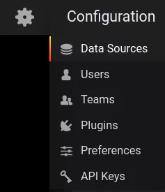
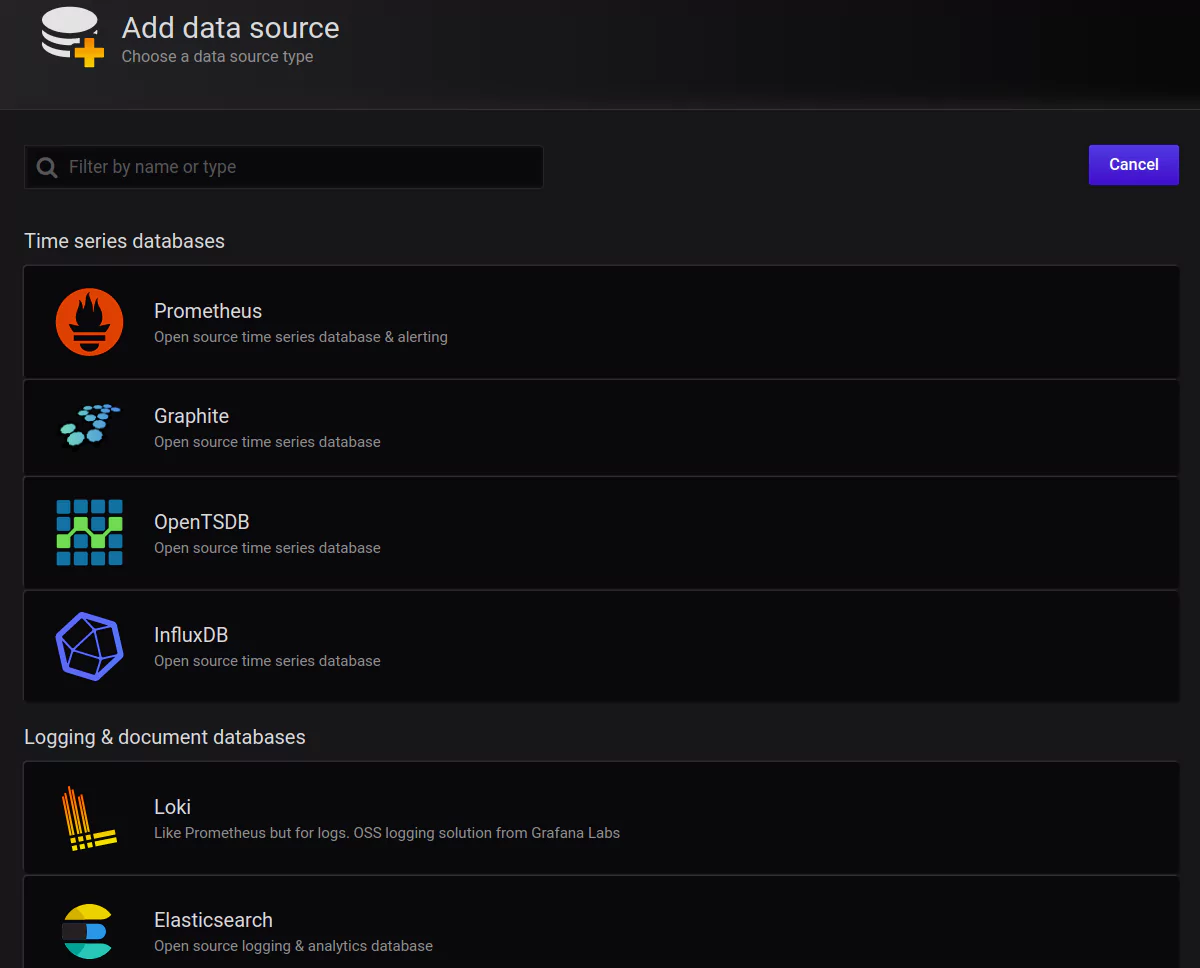
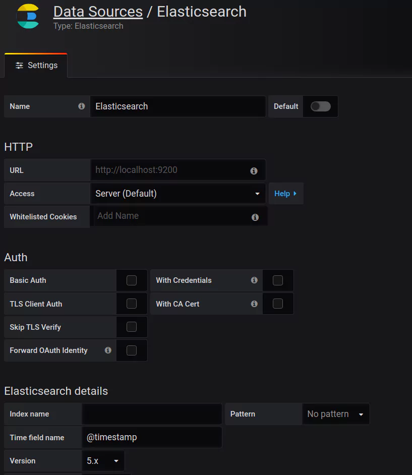
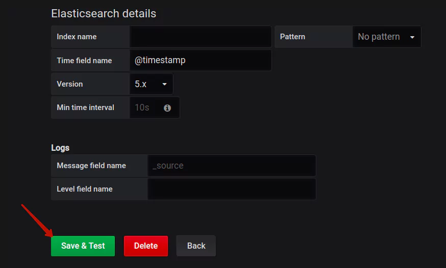
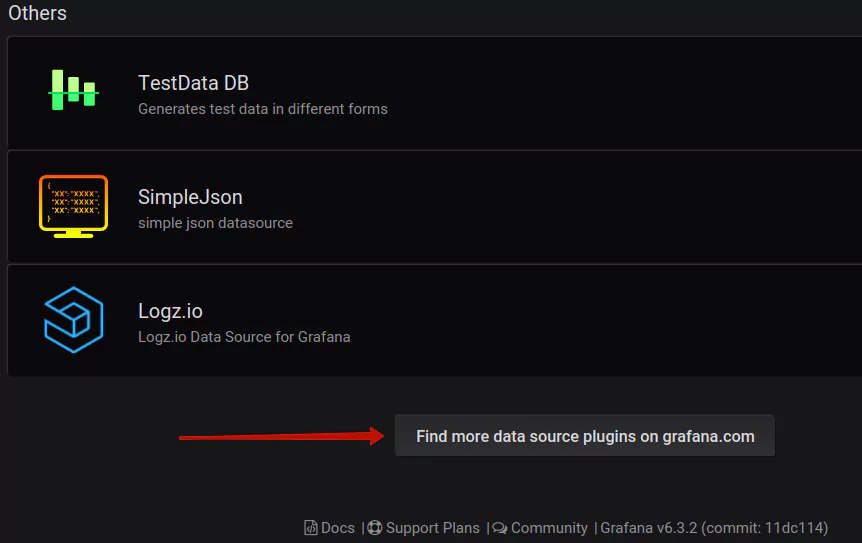
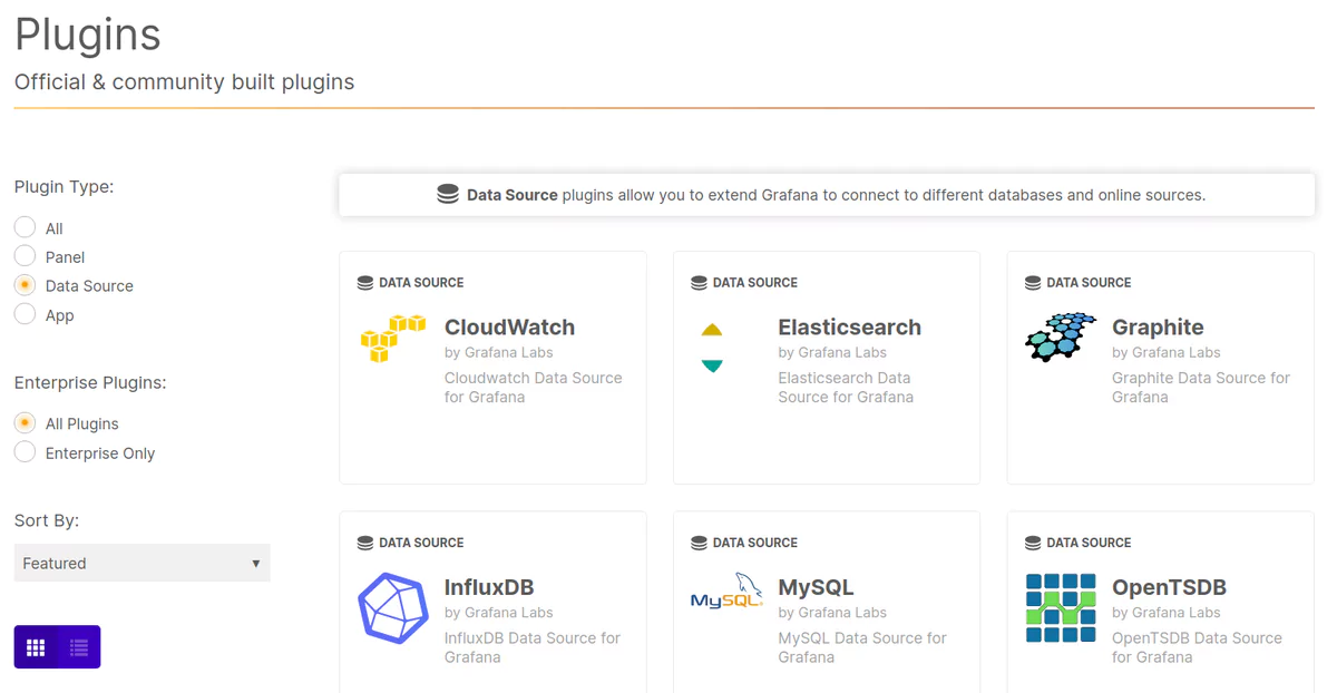
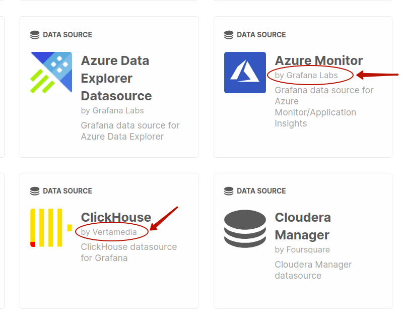
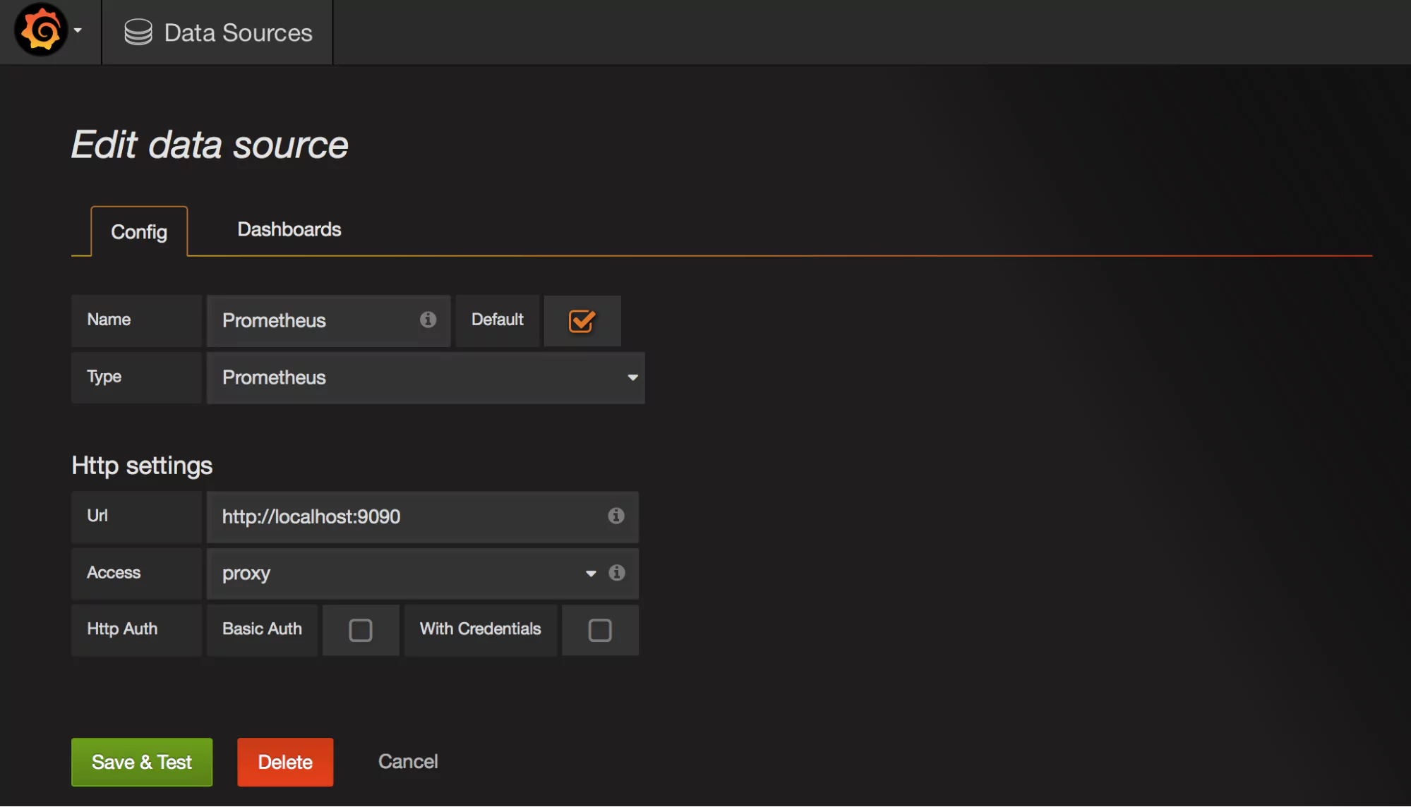
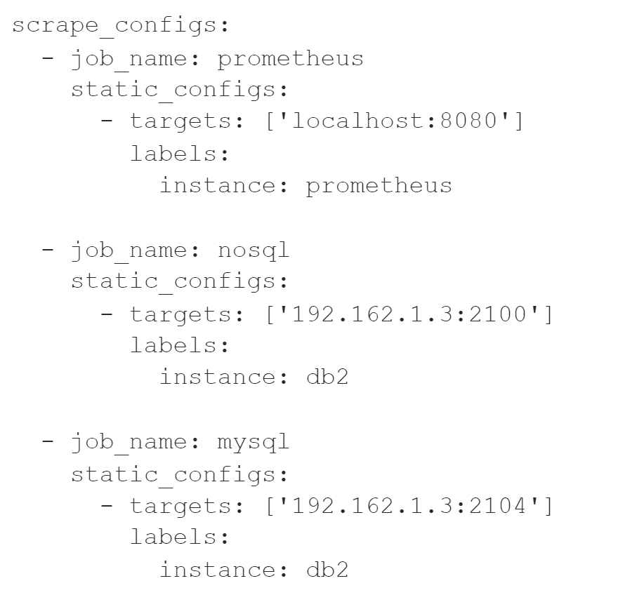
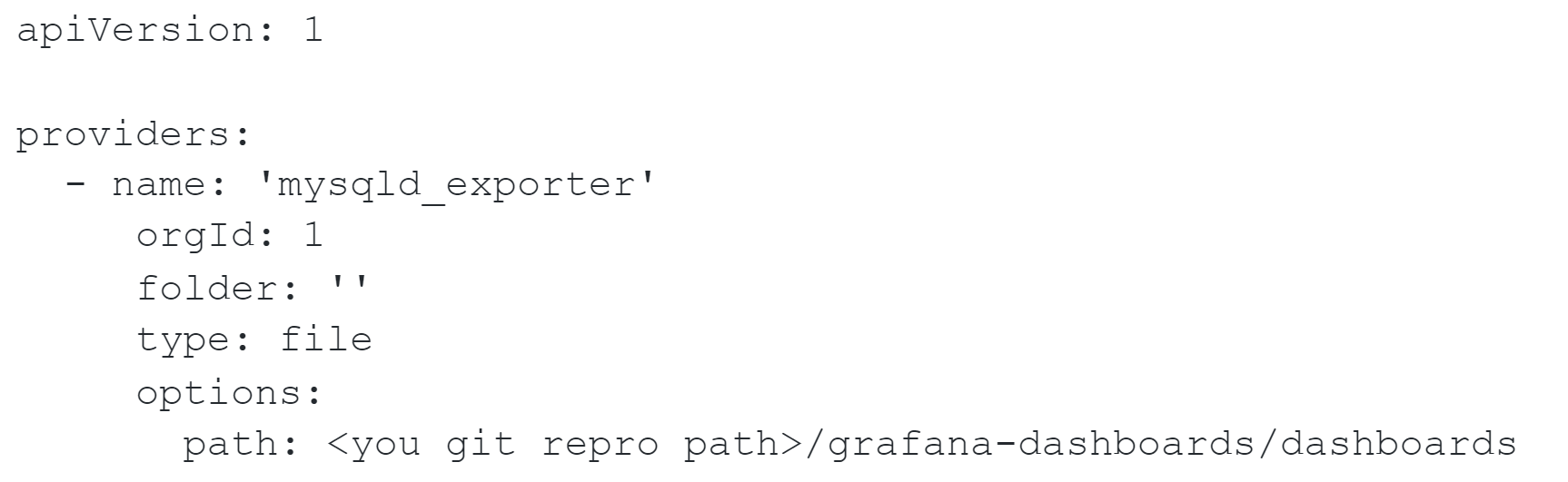
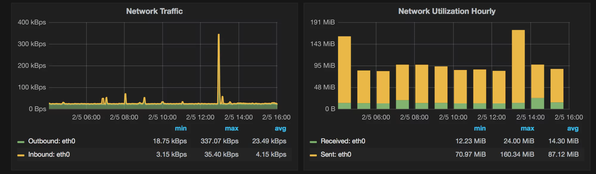
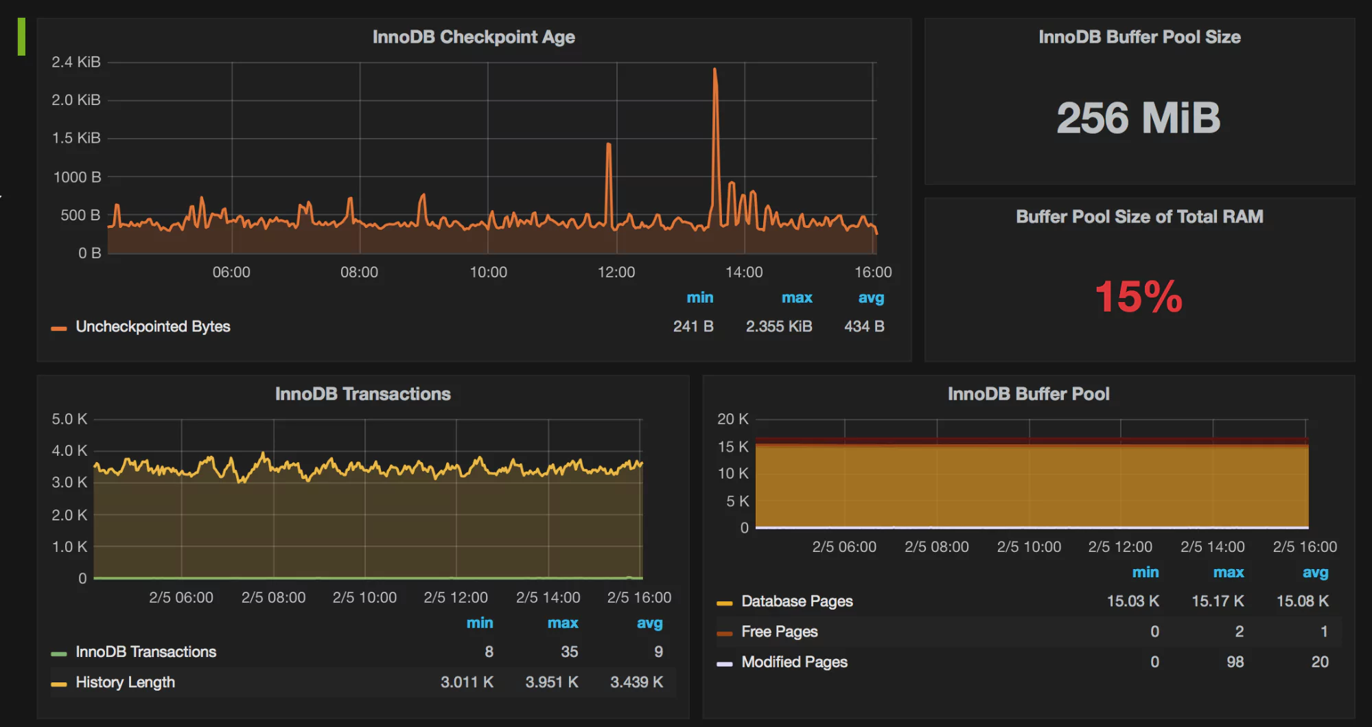
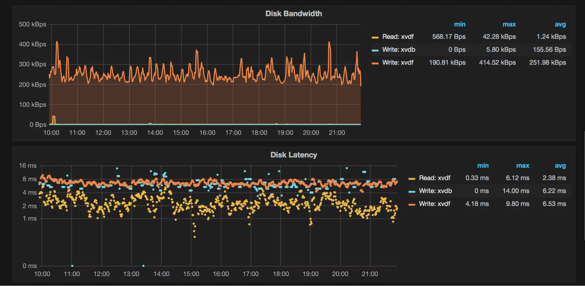
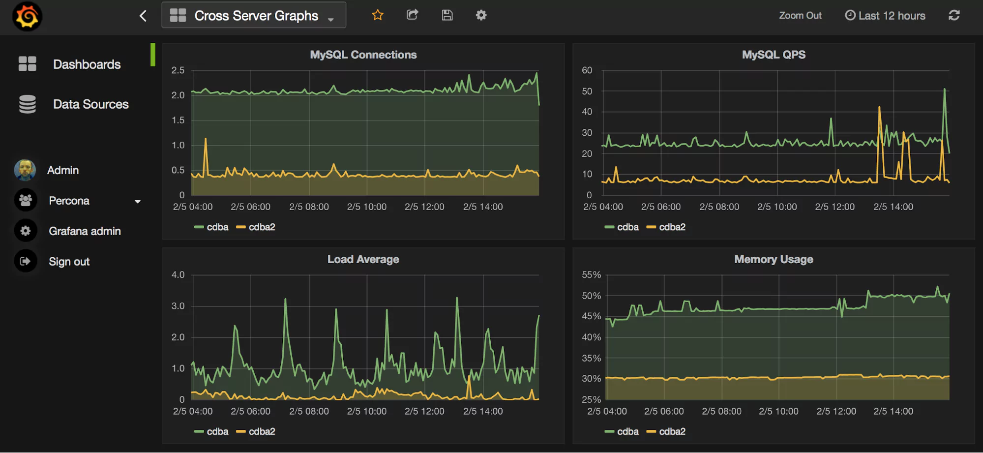
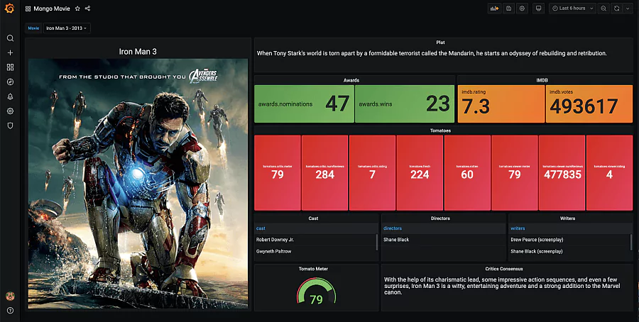
![Optimizing logs for a more effective CI/CD pipeline [Best Practices]](https://coralogix.com/wp-content/webp-express/webp-images/doc-root/wp-content/uploads/2025/06/146.png.webp)
![Heroku Continuous Integration & Deployment with Docker [Hands-On Tutorial]](https://coralogix.com/wp-content/uploads/2020/05/2-9.png)