Mapping is an essential foundation of an index that can generally be considered the heart of Elasticsearch. So you can be sure of the importance of a well-managed mapping. But just as it is with many important things, sometimes mappings can go wrong. Let’s take a look at various issues that can arise with mappings and how to deal with them.
Before delving into the possible challenges with mappings, let’s quickly recap some key points about Mappings. A mapping essentially entails two parts:
The Process: A process of defining how your JSON documents will be stored in an index
The Result: The actual metadata structure resulting from the definition process
The Process
If we first consider the process aspect of the mapping definition, there are generally two ways this can happen:
An explicit mapping process where you define what fields and their types you want to store along with any additional parameters.
A dynamic mapping Elasticsearch automatically attempts to determine the appropropriate datatype and updates the mapping accordingly.
The Result
The result of the mapping process defines what we can “index” via individual fields and their datatypes, and also how the indexing happens via related parameters.
It’s a very simple mapping example for a basic logs collection microservice. The individual logs consist of the following fields and their associated datatypes:
The actual log Message mapped as text to enable full-text searching
More… As we have not disabled the default dynamic mapping process so we’ll be able to see how we can introduce new fields arbitrarily and they will be added to the mapping automatically.
The Challenges
So what could go wrong :)?
There are generally two potential issues that many will end up facing with Mappings:
If we create an explicit mapping and fields don’t match, we’ll get an exception if the mismatch falls beyond a certain “safety zone”. We’ll explain this in more detail later.
If we keep the default dynamic mapping and then introduce many more fields, we’re in for a “mapping explosion” which can take our entire cluster down.
Let’s continue with some interesting hands-on examples where we’ll simulate the issues and attempt to resolve them.
Hands-on Exercises
Field datatypes – mapper_parsing_exception
Let’s get back to the “safety zone” we mentioned before when there’s a mapping mismatch.
We’ll create our index and see it in action. We are using the exact same mapping that we saw earlier:
Great! It worked without throwing an exception. This is the “safety zone” I mentioned earlier.
But what if that service logged a string that has no relation to numeric values at all into the Port field, which we earlier defined as an Integer? Let’s see what happens:
curl --request POST 'https://localhost:9200/microservice-logs/_doc?pretty'
--header 'Content-Type: application/json'
--data-raw '{"timestamp": "2020-04-11T12:34:56.789Z", "service": "XYZ", "host_ip": "10.0.2.15", "port": "NONE", "message": "I am not well!" }'
>>>
{
 "error" : {
   "root_cause" : [
     {
       "type" : "mapper_parsing_exception",
       "reason" : "failed to parse field [port] of type [integer] in document with id 'J5Q2anEBPDqTc3yOdTqj'. Preview of field's value: 'NONE'"
     }
   ],
   "type" : "mapper_parsing_exception",
   "reason" : "failed to parse field [port] of type [integer] in document with id 'J5Q2anEBPDqTc3yOdTqj'. Preview of field's value: 'NONE'",
   "caused_by" : {
     "type" : "number_format_exception",
     "reason" : "For input string: "NONE""
   }
 },
 "status" : 400
}
We’re now entering the world of Elastisearch mapping exceptions! We received a code 400 and the mapper_parsing_exception that is informing us about our datatype issue. Specifically that it has failed to parse the provided value of “NONE” to the type integer.
So how we solve this kind of issue? Unfortunately, there isn’t a one-size-fits-all solution. In this specific case we can “partially” resolve the issue by defining an ignore_malformed mapping parameter.
Keep in mind that this parameter is non-dynamic so you either need to set it when creating your index or you need to: close the index → change the setting value → reopen the index. Something like this.
curl --request POST 'https://localhost:9200/microservice-logs/_close'

curl --location --request PUT 'https://localhost:9200/microservice-logs/_settings'
--header 'Content-Type: application/json'
--data-raw '{
   "index.mapping.ignore_malformed": true
}'

curl --request POST 'https://localhost:9200/microservice-logs/_open'
Now let’s try to index the same document:
curl --request POST 'https://localhost:9200/microservice-logs/_doc?pretty'
--header 'Content-Type: application/json'
--data-raw '{"timestamp": "2020-04-11T12:34:56.789Z", "service": "XYZ", "host_ip": "10.0.2.15", "port": "NONE", "message": "I am not well!" }'
Checking the document by its ID will show us that the port field was omitted for indexing. We can see it in the “ignored” section.
The reason this is only a “partial” solution is because this setting has its limits and they are quite considerable. Let’s reveal one in the next example.
A developer might decide that when a microservice receives some API request it should log the received JSON payload in the message field. We already mapped the message field as text and we still have the ignore_malformed parameter set. So what would happen? Let’s see:
curl --request POST 'https://localhost:9200/microservice-logs/_doc?pretty'
--header 'Content-Type: application/json'
--data-raw '{"timestamp": "2020-04-11T12:34:56.789Z", "service": "ABC", "host_ip": "10.0.2.15", "port": 12345, "message": {"data": {"received":"here"}}}'
>>>
{
...
       "type" : "mapper_parsing_exception",
       "reason" : "failed to parse field [message] of type [text] in document with id 'LJRbanEBPDqTc3yOjTog'. Preview of field's value: '{data={received=here}}'"
...
}
We see our old friend, the mapper_parsing_exception! This is because ignore_malformedcan’t handle JSON objects on the input. Which is a significant limitation to be aware of.
Now, when speaking of JSON objects be aware that all the mapping ideas remains valid for their nested parts as well. Continuing our scenario, after losing some logs to mapping exceptions, we decide it’s time to introduce a new payload field of the type object where we can store the JSON at will.
Remember we have dynamic mapping in place so you can index it without first creating its mapping:
It was mapped as an object with (sub)properties defining the nested fields. So apparently the dynamic mapping works! But there is a trap. The payloads (or generally any JSON object) in the world of many producers and consumers can consist of almost anything. So you know what will happen with different JSON payload which also consists of a payload.data.received field but with a different type of data:
Engineers on the team need to be made aware of these mapping mechanics. You can also eastablish shared guidelines for the log fields.
Secondly you may consider what’s called a Dead Letter Queue pattern that would store the failed documents in a separate queue. This either needs to be handled on an application level or by employing Logstash DLQ which allows us to still process the failed documents.
Limits – illegal_argument_exception
Now the second area of caution in relation to mappings, are limits. Even from the super-simple examples with payloads you can see that the number of nested fields can start accumulating pretty quickly. Where does this road end? At the number 1000. Which is the default limit of the number of fields in a mapping.
Let’s simulate this exception in our safe playground environment before you’ll unwillingly meet it in your production environment.
We’ll start by creating a large dummy JSON document with 1001 fields, POST it and then see what happens.
To create the document, you can either use the example command below with jq tool (apt-get install jq if you don’t already have it) or create the JSON manually if you prefer:
curl --location --request PUT 'https://localhost:9200/big-objects'
And if we then POST our generated JSON, can you guess what’ll happen?
curl --request POST 'https://localhost:9200/big-objects/_doc?pretty'
--header 'Content-Type: application/json'
--data-raw "$thousandone_fields_json"
>>>
{
 "error" : {
   "root_cause" : [
     {
       "type" : "illegal_argument_exception",
       "reason" : "Limit of total fields [1000] in index [big-objects] has been exceeded"
     }
...
 "status" : 400
}
… straight to the illegal_argument_exception exception! This informs us about the limit being exceeded.
So how do we handle that? First, you should definitely think about what you are storing in your indices and for what purpose. Secondly, if you still need to, you can increase this 1,000 limit. But be careful as with bigger complexity might come a much bigger price of potential performance degradations and high memory pressure (see the docs for more info).
Changing this limit can be performed with a simple dynamic setting change:
In this Hadoop Tutorial lesson, we’ll learn how we can use Elasticsearch Hadoop to process very large amounts of data. For our exercise, we’ll use a simple Apache access log to represent our “big data”. We’ll learn how to write a MapReduce job to ingest the file with Hadoop and index it into Elasticsearch.
What Is Hadoop?
When we need to collect, process/transform, and/or store thousands of gigabytes of data, thousands of terabytes, or even more, Hadoop can be the appropriate tool for the job. It is built from the ground up with ideas like this in mind:
Use multiple computers at once (forming a cluster) so that it can process data in parallel, to finish the job much faster. We can think of it this way. If one server needs to process 100 terabytes of data, it might finish in 500 hours. But if we have 100 servers, each one can just take a part of the data, for example, server1 can take the first terabyte, server2 can take the second terabyte, and so on. Now they each have only 1 terabyte to process and they can all work on their own section of data, at the same time. This way, the job can be finished in 5 hours instead of 500. Of course, this is theoretical and imaginary, as in practice we won’t get a 100 times reduction in the time it takes, but we can get pretty close to that if conditions are ideal.
Make it very easy to adjust the computing power when needed. Have a lot more data to process, and the problem is much more complex? Add more computers to the cluster. In a sense, it’s like adding more CPU cores to a supercomputer.
Data grows and grows, so Hadoop must be able to easily and flexibly expand its storage capacity too, to keep up with demand. Every computer we add to the cluster expands the total storage space available to the Hadoop Distributed File System (HDFS).
Unlike other software, it doesn’t just try to recover from hardware failure when it happens. The design philosophy actually assumes that some hardware will certainly fail. When having thousands of computers, working in parallel, it’s guaranteed that something, somewhere, will fail, from time to time. As such, Hadoop, by default, creates replicas of chunks of data and distributes them on separate hardware, so nothing should be lost when the occasional server goes up in flames or a hard-disk or SSD dies.
To summarize, Hadoop is very good at ingesting and processing incredibly large volumes of information. It distributes data across the multiple nodes available in the cluster and uses the MapReduce programming model to process it on multiple machines at once (parallel processing).
But this may sound somewhat similar to what Elasticsearch data ingestion tools do. Although they’re made to deal with rather different scenarios, they may sometimes overlap a bit. So why and when would we use one instead of the other?
Hadoop vs Logstash/Elasticsearch
First of all, we shouldn’t think in terms of which one is better than the other. Each excels at the jobs it’s created for. Each has pros and cons.
To try to paint a picture and give you an idea of when we’d use one or the other, let’s think of these scenarios:
When we’d need to ingest data from billions of websites, as a search engine like Google does, we’d find a tool like Elasticsearch Hadoop very useful and efficient.
When we need to store data and index it in such a way that it can later be searched quickly and efficiently, we’ll find something like Elasticsearch very useful.
And, finally, when we want to gather real time data, like the price of USD/EUR from many exchanges available on the Internet, we’d find a tool like Logstash is good for the job.
Of course, if the situation allows it, Hadoop and Elasticsearch can also be teamed up, so we can get the best of both worlds. Remember the scenario of scanning information on billions of websites? Hadoop would be great at collecting all that data, and send it to be stored in Elasticsearch. Elasticsearch would then be great at quickly returning results to the users that search through that data.
With Elasticsearch, you can think: awesome search capabilities, good enough in the analytics and data visualization department.
With Elasticsearch Hadoop, you can think: capable of ingesting and processing mind-blowing amounts of data, in a very efficient manner, and allow for complex, fine-tuned data processing.
How MapReduce Works
As mentioned, while tools like Logstash or even Spark are easier to use, they also confine us to the methods they employ. That is, we can only fine-tune the settings they allow us to adjust and we can’t change how their programming logic works behind the scenes. That’s not usually a problem, as long as we can do what we want.
With Hadoop, however, we have more control over how things work at a much lower level, allowing for much more customization and more importantly, optimization. When we deal with petabytes of data, optimization can matter a lot. It can help us reduce the time needed for a job, from months to weeks, and significantly reduce operation costs and resources needed.
Let’s take a first look at MapReduce, which adds complexity to our job but also allows for the higher level of control mentioned earlier.
A MapReduce procedure typically consists of three main stages: Map, Shuffle and Reduce.
Initially, data is split into smaller chunks that can be spread across different computing nodes. Next, every node can execute a map task on its received chunk of data. This kind of parallel processing greatly speeds up the procedure. The more nodes the cluster has, the faster the job can be done.
Pieces of mapped data, in the form of key/value pairs, now sit on different servers. All the values with the same key need to be grouped together. This is the shuffle stage. Next, shuffled data goes through the reduce stage.
This image exemplifies these stages in action on a collection of three lines of words.
Here, we assume that we have a simple text file and we need to calculate the number of times each word appears within.
The first step is to read the data and split it into chunks that can be efficiently sent to all processing nodes. In our case, we assume the file is split into three lines.
Map Stage
Next comes the Map stage. Lines are used as input for the map(key, value, context) method. This is where we’ll have to program our desired custom logic. For this word count example, the “value” parameter will hold the line input (line of text from file). We’ll then split the line, using the space character as a word separator, then iterate through each of the splits (words) and emit a map output using context.write(key, value). Here, our key will be the word, for example, “Banana” and the value will be 1, indicating it’s a single occurrence of the word. From the image above we can see that for the first line we get <Banana, 1>, <Apple, 1>, <Mango, 1> as key/value pairs.
Shuffle Stage
The shuffle stage is responsible for taking <key, value> pairs from the mapper, and, based on a partitioner, decide to which reducer each goes to.
From the image showing each stage in action, we can see that we end up with five partitions in the reduce stage. Shuffling is done internally by the framework, so we will not have any custom code for that here.
Reduce Stage
The output of the shuffle stage is fed into the reduce stage: as its input, each reducer receives one of the groups formed in the shuffle stage. This consists of a key and a list of values related to the key. Here, we again have to program custom logic we want to be executed in this stage. In this example, for every key, we have to calculate the sum of the elements in its value list. This way, we get the total count of each key, which ultimately represents the count for each unique word in our text file.
The output of the reduce stage also follows the <key, value> format. As mentioned, in this example, the key will represent the word and the value the number of times the word has been repeated.
Hands-On Exercise
OpenJDK Prerequisite
Wow! There’s a lot of theory behind Hadoop, but practice will help us cement the concepts and understand everything better.
Let’s learn how to set up a simple Hadoop installation.
Since Elasticsearch is already installed, the appropriate Java components are already installed too. We can verify with:
java -version
This should show us an output similar to this:
openjdk version "11.0.7" 2020-04-14
OpenJDK Runtime Environment (build 11.0.7+10-post-Ubuntu-2ubuntu218.04)
OpenJDK 64-Bit Server VM (build 11.0.7+10-post-Ubuntu-2ubuntu218.04, mixed mode, sharing)
OpenJDK is required by Hadoop and on an instance where this is not available, you can install it with a command such as “sudo apt install default-jdk”.
Create a Hadoop User
Now let’s create a new user, called “hadoop”. Hadoop related processes, such as the MapReduce code we’ll use, will run under this user. Remember the password you set for this user, as it’s needed later, when logging in, and using sudo commands while logged in.
sudo adduser hadoop
We’ll add the user to the sudo group, to be able to execute some later commands with root privileges.
sudo usermod -aG sudo hadoop
Let’s log in as the “hadoop” user.
su - hadoop
Install Hadoop Binaries
Note: For testing purposes commands below can be left unchanged. On production systems, however, you should first visit https://www.apache.org/dyn/closer.cgi/hadoop/common/stable and find out which Hadoop version is the latest stable one. Afterward, you will need to modify “https” links to point to the latest stable version and change text strings containing “hadoop-3.2.1” in commands used below to whatever applies to you (as in, change “3.2.1” version number to current version number). It’s a very good idea to also follow instructions regarding verifying integrity of downloads with GPG (verify signatures).
While logged in as the Hadoop user, we’ll download the latest stable Hadoop distribution using the wget command.
Next, let’s extract the files from the tar archive compressed with gzip.
tar -xvzf hadoop-3.2.1.tar.gz
Once this is done, we’ll move the extracted directory to “/usr/local/hadoop/”.
sudo mv hadoop-3.2.1 /usr/local/hadoop
With the method we followed, the “/usr/local/hadoop” directory should already be owned by the “hadoop” user and group. But to make sure this is indeed owned by this user and group, let’s run the next command.
sudo chown -R hadoop:hadoop /usr/local/hadoop
Hadoop uses environment variables to orient itself about the directory paths it should use. Let’s set these variables according to our setup.
nano ~/.bashrc
Let’s scroll to the end of the file and add these lines:
To quit the nano editor and save our file we’ll first press CTRL+X, then type “y” and finally press ENTER.
To make the environment variables specified in the “.bashrc” file take effect, we’ll use:
source ~/.bashrc
Configure Hadoop Properties
Hadoop needs to know where it can find the Java components it requires. We point it to the correct location by using the JAVA_HOME environment variable.
Let’s see where the “javac” binary is located:
readlink -f $(which javac)
In the case of OpenJDK 11, this will point to “/usr/lib/jvm/java-11-openjdk-amd64/bin/javac“.
We’ll need to copy the path starting with “/usr” and ending with “openjdk-amd64“, which means we exclude the last part: “/bin/javac” in this case.
In the case of OpenJDK 11, the path we’ll copy is:
/usr/lib/jvm/java-11-openjdk-amd64
and we’ll paste it at the end of the last line: export JAVA_HOME=
Let’s open the “hadoop-env.sh” file in the nano editor and add this path to the JAVA_HOME variable.
sudo nano $HADOOP_HOME/etc/hadoop/hadoop-env.sh
We’ll scroll to the end of the file and add this line:
Remember, if the OpenJDK version you’re using is different, you will need to paste a different string of text after “export JAVA_HOME=“.
Once again, we’ll press CTRL+X, then type “y” and finally press ENTER to save the file.
Let’s test if our setup is in working order.
hadoop version
We should see an output similar to this
Hadoop 3.2.1
Source code repository https://gitbox.apache.org/repos/asf/hadoop.git -r b3cbbb467e22ea829b3808f4b7b01d07e0bf3842
Compiled by rohithsharmaks on 2019-09-10T15:56Z
Compiled with protoc 2.5.0
From source with checksum 776eaf9eee9c0ffc370bcbc1888737
This command was run using /usr/local/hadoop/share/hadoop/common/hadoop-common-3.2.1.jar
Creating MapReduce Project
In this exercise, we’ll index a sample access log file which was generated in the Apache Combined Log Format. We’ll use the maven build tool to compile our MapReduce code into a JAR file.
In a real scenario, you would have to follow a few extra steps:
Install an integrated development environment (IDE) that includes a code editor, such as Eclipse, to create a project and write the necessary code.
Compile project with maven, on local desktop.
Transfer compiled project (JAR), from local desktop to your Hadoop instance.
We’ll explain the theory behind how you would create such a project, but we’ll also provide a GitHub repository containing a ready-made, simple Java project. This way, you don’t have to waste time writing code for now, and can just start experimenting right away and see MapReduce in action. Furthermore, if you’re unfamiliar with Java programming, you can take a look at the sample code to better understand where all the pieces go and how they fit.
So, first, let’s look at the theory and see how we would build MapReduce code, and what is the logic behind it.
Setting Up pom.xml Dependencies
To get started, we would first have to create an empty Maven project using the code editor we prefer. Both Eclipse and IntelliJ have built-in templates to do this. We can skip archetype selection when creating the maven project; an empty maven project is all we require here.
Once the project is created, we would edit the pom.xml file and use the following properties and dependencies. Some versions numbers specified below may need to be changed in the future, when new stable versions of Hadoop and Elasticsearch are used.
The hadoop-client library is required to write MapReduce Jobs. In order to write to an Elasticsearch index we are using the official elasticsearch-hadoop-mr library. commons-httpclient is needed too, because elasticsearch-hadoop-mr uses this to be able to make REST calls to the Elasticsearch server, through the HTTP protocol.
Defining the Logic of Our Mapper Class
We’ll define AccessLogMapper and use it as our mapper class. Within it, we’ll override the default map() method and define the programming logic we want to use.
import org.apache.hadoop.mapreduce.Mapper;
import java.io.IOException;

public class AccessLogIndexIngestion {

   public static class AccessLogMapper extends Mapper {
       @Override
       protected void map(Object key, Object value, Context context) throws IOException, InterruptedException {
       }
   }

   public static void main(String[] args) {

   }
}
As mentioned before, we don’t need a reducer class in this example.
We’ve dealt with theory only up to this point, but here, it’s important we execute the next command.
Let’s send this curl request to define the index in Elasticsearch. For the purpose of this exercise, we ignore the last two columns in the log in this index structure.
Having the dateTime field defined as a date is essential since it will enable us to visualize various metrics using Kibana. Of course, we also needed to specify the date/time format used in the access log, “dd/MMM/yyyy:HH:mm:ss”, so that values passed along to Elasticsearch are parsed correctly.
Defining map() Logic
Since our input data is a text file, we use the TextInputFormat.class. Every line of the log file will be passed as input to the map() method.
Finally, we can define the core logic of the program: how we want to process each line of text and get it ready to be sent to the Elasticsearch index, with the help of the EsOutputFormat.class.
The value input parameter of the map() method holds the line of text currently extracted from the log file and ready to be processed. We can ignore the key parameter for this simple example.
import org.elasticsearch.hadoop.util.WritableUtils;
import org.apache.hadoop.io.NullWritable;
import java.io.IOException;
import java.util.LinkedHashMap;
import java.util.Map;

@Override
protected void map(Object key, Object value, Context context) throws IOException, InterruptedException {

   String logEntry = value.toString();
   // Split on space
   String[] parts = logEntry.split(" ");
   Map<String, String> entry = new LinkedHashMap<>();

   // Combined LogFormat "%h %l %u %t "%r" %>s %b "%{Referer}i" "%{User-agent}i"" combined
   entry.put("ip", parts[0]);
   // Cleanup dateTime String
   entry.put("dateTime", parts[3].replace("[", ""));
   // Cleanup extra quote from HTTP Status
   entry.put("httpStatus", parts[5].replace(""",  ""));
   entry.put("url", parts[6]);
   entry.put("responseCode", parts[8]);
   // Set size to 0 if not present
   entry.put("size", parts[9].replace("-", "0"));
   context.write(NullWritable.get(), WritableUtils.toWritable(entry));
}
We split the line into separate pieces, using the space character as a delimiter. Since we know that the first column in the log file represents an IP address, we know that parts[0] holds such an address, so we can prepare that part to be sent to Elasticsearch as the IP field. Similarly, we can send the rest of the columns from the log, but some of them need special processing beforehand. For example, when we split the input string, using the space character as a delimiter, the time field got split into two entries, since it contains a space between the seconds number and timezone (+0000 in our log). For this reason, we need to reassemble the timestamp and concatenate parts 3 and 4.
The EsOutputFormat.class ignores the “key” of the Mapper class output, hence in context.write() we set the key to NullWriteable.get()
MapReduce Job Configuration
We need to tell our program where it can reach Elasticsearch and what index to write to. We do that with conf.set(“es.nodes”, “localhost:9200”); and conf.set(“es.resource”, “logs”);.
Under normal circumstances, speculative execution in Hadoop can sometimes optimize jobs. But, in this case, since output is sent to Elasticsearch, it might accidentally cause duplicate entries or other issues. That’s why it’s recommended to disable speculative execution for such scenarios. You can read more about this, here: https://www.elastic.co/guide/en/elasticsearch/hadoop/current/configuration-runtime.html#_speculative_execution. These lines disable the feature:
Since the MapReduce job will essentially read a text file in this case, we use the TextInputFormat class for our input: job.setInputFormatClass(TextInputFormat.class);
And, since we want to write to an Elasticsearch index, we use the EsOutputFormat class for our output: job.setOutputFormatClass(EsOutputFormat.class);
Next, we set the Mapper class we want to use, to the one we created in this exercise: job.setMapperClass(AccessLogMapper.class);
And, finally, since we do not require a reducer, we set the number of reduce tasks to zero: job.setNumReduceTasks(0);
Building the JAR File
Once all the code is in place, we have to build an executable JAR. For this, we use the maven-shade-plugin, so we would add the following to “pom.xml“.
Now let’s copy the JAR file we compiled earlier, to the same location where our access log is located (include the last dot “.” in this command, as that tells the copy command that “destination is current location”).
cp target/eswithmr-1.0-SNAPSHOT.jar .
Finally, we can execute the MapReduce job.
hadoop jar eswithmr-1.0-SNAPSHOT.jar access.log
When the job is done, the last part of the output should look similar to this:
File System Counters
		FILE: Number of bytes read=2370975
		FILE: Number of bytes written=519089
		FILE: Number of read operations=0
		FILE: Number of large read operations=0
		FILE: Number of write operations=0
	Map-Reduce Framework
		Map input records=10000
		Map output records=10000
		Input split bytes=129
		Spilled Records=0
		Failed Shuffles=0
		Merged Map outputs=0
		GC time elapsed (ms)=33
		Total committed heap usage (bytes)=108003328
	File Input Format Counters
		Bytes Read=2370789
	File Output Format Counters
		Bytes Written=0
	Elasticsearch Hadoop Counters
		Bulk Retries=0
		Bulk Retries Total Time(ms)=0
		Bulk Total=10
		Bulk Total Time(ms)=1905
		Bytes Accepted=1656164
		Bytes Received=40000
		Bytes Retried=0
		Bytes Sent=1656164
		Documents Accepted=10000
		Documents Received=0
		Documents Retried=0
		Documents Sent=10000
		Network Retries=0
		Network Total Time(ms)=2225
		Node Retries=0
		Scroll Total=0
		Scroll Total Time(ms)=0
We should pay close attention to the Map-Reduce Framework section. In this case, we can see everything went according to plan: we had 10.000 input records and we got 10.000 output records.
To verify the records are indexed into Elasticsearch, let’s run the following command:
curl 'localhost:9200/_cat/indices?v'
We should see a docs.count matching the number of records, 10.000 in this case.
health status index uuid               	pri rep docs.count docs.deleted store.size pri.store.size
yellow open   logs  WEPWCieYQXuIRp2LlZ_QIA   1   1  	10000        	0  	1.1mb      	1.1mb
After clicking on “Next step“, from the drop-down list titled “Time Filter field name” we choose “dateTime” and then click on “Create index pattern“.
We’ll land on a screen like this:
Visualize Data in Kibana
In the left side menu, let’s navigate to the Discover page.
Now let’s set the time range from 16th of May to 21st of May 2015 and then click the “Update” button.
The visualized data should look like this:
From the “Available fields” section on the left, highlight “httpStatus”, “url” and “size“, and hit the “Add” button that appears next to them. Now we only see the metrics we’re interested in and get much cleaner output.
Filtering Data in Kibana
Since we have set the “size” property of the index to be of type integer, we can run filters based on the size. Let’s view all requests which returned data larger than 5MB.
In the Search box above, type
size >= 5000000
and press ENTER.
Above the bar chart, we can click on the drop-down list displaying “Auto” and change that time interval to “Hourly“. Now each bar displayed represents data collected in one hour.
Clean Up Steps
Let’s remove the index we have created in this lesson:
curl -XDELETE 'localhost:9200/logs'
In the terminal window where we are still logged in as the “hadoop” user, we can also remove the files we created, such as the JAR file, the Java code, access log, and so on. Of course, if you want to keep them and continue experimenting, you can skip the next command.
To remove all the files, we run:
cd && rm -rf elasticsearch-with-hadoop-mr-lesson/
And, finally, we remove the Hadoop installation archive:
rm hadoop-3.2.1.tar.gz
Conclusion
These are the basic concepts behind writing, compiling and executing MapReduce jobs with Hadoop. Although setting up a multi-node cluster is a much more complex operation, the concepts behind creating a MapReduce algorithm and running it, in parallel, on all the computers in the cluster, instead of a single machine, remain almost the same.
Source Code
package com.coralogix

import org.apache.hadoop.conf.Configuration;
import org.apache.hadoop.fs.Path;
import org.apache.hadoop.io.NullWritable;
import org.apache.hadoop.mapreduce.Job;
import org.apache.hadoop.mapreduce.Mapper;
import org.apache.hadoop.mapreduce.lib.input.FileInputFormat;
import org.apache.hadoop.mapreduce.lib.input.TextInputFormat;
import org.elasticsearch.hadoop.mr.EsOutputFormat;
import org.elasticsearch.hadoop.util.WritableUtils;

import java.io.IOException;
import java.util.LinkedHashMap;
import java.util.Map;

public class AccessLogIndexIngestion {

   public static class AccessLogMapper extends Mapper {
       @Override
       protected void map(Object key, Object value, Context context) throws IOException, InterruptedException {

           String logEntry = value.toString();
           // Split on space
           String[] parts = logEntry.split(" ");
           Map<String, String> entry = new LinkedHashMap<>();

           // Combined LogFormat "%h %l %u %t "%r" %>s %b "%{Referer}i" "%{User-agent}i"" combined
           entry.put("ip", parts[0]);
           // Cleanup dateTime String
           entry.put("dateTime", parts[3].replace("[", ""));
           // Cleanup extra quote from HTTP Status
           entry.put("httpStatus", parts[5].replace(""",  ""));
           entry.put("url", parts[6]);
           entry.put("responseCode", parts[8]);
           // Set size to 0 if not present
           entry.put("size", parts[9].replace("-", "0"));

           context.write(NullWritable.get(), WritableUtils.toWritable(entry));
       }
   }

   public static void main(String[] args) throws IOException, ClassNotFoundException, InterruptedException {
       Configuration conf = new Configuration();
       conf.setBoolean("mapred.map.tasks.speculative.execution", false);
       conf.setBoolean("mapred.reduce.tasks.speculative.execution", false);
       conf.set("es.nodes", "localhost:9200");
       conf.set("es.resource", "logs");

       Job job = Job.getInstance(conf);
       job.setInputFormatClass(TextInputFormat.class);
       job.setOutputFormatClass(EsOutputFormat.class);
       job.setMapperClass(AccessLogMapper.class);
       job.setNumReduceTasks(0);

       FileInputFormat.addInputPath(job, new Path(args[0]));
       System.exit(job.waitForCompletion(true) ? 0 : 1);
   }

}
If our end users end up too long for a query to return results due to Elasticsearch query performance issues, it can often lead to frustration. Slow queries can affect the search performance of an ecommerce site or a Business Intelligence dashboard – either way, this could lead to negative business consequences. So it’s important to know how to monitor the speed of search queries, diagnose and debug to improve search performance.
We have two main tools at our disposal to help us investigate and optimize the speed of Elasticsearch queries: Slow Log and Search Profiling.
Let’s review the features of these two instruments, examine a few use cases, and then test them out in our sandbox environment.
With sufficiently complex data it can be difficult to anticipate how end users will interact with your system. We may not have a clear idea of what they are searching for, and how they perform these searches. Because of this, we need to monitor searches for anomalies that may affect the speed of applications in a production environment. The Slow Log captures queries and their related metadata when a specified processing time exceeds a threshold for specific shards in a cluster.
Slow Log
Here’s a sample slow log entry is as follows:
[2020-04-18T12:34:56,789][WARN ][i.s.s.fetch ] [### NODE NAME ###] [### INDEX ####][0] took[### TIME IN SEC ###], took_millis[### TIME IN MS ###], total_hits[### NUM OF HITS ###], types[], stats[], search_type[QUERY_THEN_FETCH], total_shards[1], source[{ ### THE SOURCE QUERY ### }], id[ #### ID OF A USER #### ],
Data in these logs consists of:
Timestamp when the query was executed (for instance, for tracking the time of day of certain issues)
Node ID
Name of the index where it was executed and how long it took
Query in the source field
The Slow Log also has a JSON version, making it possible to fetch these logs into Elasticsearch for analysis and displaying in a dashboard.
Search Profiling
When you discover Elasticsearch query performance issues in the Slow Log, you can analyze both the search queries and aggregations with the Profile API. The execution details are a fundamental aspect of Apache Lucene which lies under the hood of every shard, so let’s explore the key pieces and principles of the profiling output.
Let’s break down the response from the Profile API when it’s enabled on a search query:
PROFILE → the root object consisting of the full profiling payload.
array
SHARD → the profile is separated for each shard that took part in the query (we will be testing on a single-node single-shard config).
array
SEARCH → each query translates to a search entity that is processed in Lucene (Note: in most cases there will only be one).
array
QUERY → these are the individual Lucene queries that were executed. Important: these are usually not mapped 1:1 to the original Elasticsearch query, as the structure of Lucene queries is different. For example: a match query on two terms (e.g. “hello world”) will be translated to one boolean query with two term queries in Lucene.
object
BREAKDOWN → individual metrics that cover timing of various execution methods in the Lucene index and the count of how many times they were executed. These can include scoring of a document, getting a next matching document etc.
array
CHILDREN → the overall query structure may be nested. You will find a breakdown for each child in this section.
value
REWRITE_TIME → as mentioned earlier, the Elasticsearch query undergoes a “translation” process into optimal queries for Lucene to execute. This process can have many iterations; the overall time is captured here.
array
COLLECTOR → the coordination process is performed by one or more Collectors. It provides a collection of matching documents, and performs additional aggregations, counting, sorting, or filtering on the result set. Here you find the time of execution for each process.
array
AGGREGATIONS → includes the profiling details if the request consists of one or more aggregations.
object
BREAKDOWN → individual metrics that cover the aggregation details (such as initializing the aggregation, collecting the documents etc.). Note: the reduction phase is a summary of activity across shards.
array
CHILDREN → like queries, aggregations can be nested.
There’s two important points to keep in mind with Search Profiling:
These are not end-to-end measurements but only capture shard-level processing. The coordinating node work is not included, nor is any network latency, etc.
Because profiling is a debugging tool it has a very large overhead so it’s typically enabled for a limited time to debug.
Search profiling can also be visualized in Kibana DevTools for easier analysis of the profiling responses. We’ll examine this later in the hands-on section.
Hands-on: Solving Elasticsearch Query Performance
First we need some data to play with. We’ll use a data set including the Wikipedia page data provided on the Coralogix github (more info on this dataset can be found in this article). While this is not a particularly small dataset (100 Mb), it still won’t reach the scale that you’re likely to find in many real-world applications which can consist of tens of GBs, or more.
To download the data and index them into our new wiki index, follow the commands below.
mkdir profiling && cd "$_"

for i in {1..10}
do
   wget "https://raw.githubusercontent.com/coralogix-resources/wikipedia_api_json_data/master/data/wiki_$i.bulk"
done

curl --request PUT 'https://localhost:9200/wiki'
--header 'Content-Type: application/json'
-d '{"settings": { "number_of_shards": 1, "number_of_replicas": 0 }}'

for bulk in *.bulk
do
   curl --silent --output /dev/null --request POST "https://localhost:9200/wiki/_doc/_bulk?refresh=true" --header 'Content-Type: application/x-ndjson' --data-binary "@$bulk"
   echo "Bulk item: $bulk INDEXED!"
done
As you can see we are not defining a specific mapping; we are using the defaults. We will then loop through the 10 bulk files downloaded from the repo and use the _bulk API to index them.
You can get a sense of what this dataset is about with the following query:
For the slow log, we can customize a threshold that triggers a slow log to be stored with the following dynamic settings (dynamic means that you can effectively change them without restarting the index).
You can define standard log levels (warn/info/debug/trace) and also separate the query phase (documents matching and scoring) from the fetch phase (retrieval of the docs).
Notice that the profile parameter is set to true. In this query, we’re searching for “cloud services.” We want to see them appear higher in the results than those that are related to “databases.” We also do not want results with a timestamp older than a year.
As you can see in the results, the original query was rewritten to a different structure but with the shared common boolean query.
For us, the most important result is the quantity. We can see that the most costly search was the phrase query. This makes sense because it searches for the specific sequence of terms in all of the relevant docs. (Note: we have also added the slop parameter of 2 which allows for up to two other terms to appear between the queried terms).
Next let’s breakdown some of these queries. For instance, let’s examine the match phrase query:
You can see that the most costly phase seems to be the build_scorer, which is a method for scoring the documents. The matching of documents (match phase) follows close after. In most cases these low level results are not the most meaningful for us. This is because we are running in a “lab” environment with a small amount of data. These numbers become much more significant in a production environment.
Profiling – Kibana
To see everything we have discussed but in a nice visualized format, you can try the related section in Kibana Dev Tools.
You have two options for using this feature:
Copy a specific query (or an aggregation) into the text editor area and execute the profiling. (Note: don’t forget to limit the execution to a single index; otherwise the profiler will run on all).
Or, if you have a few pre-captured profiling results you can copy these into the text editor as well; the profiler will recognize that it is already a profiling output and visualize the results for you.
Try the first option with a new query so you can practice your new skills.
For the second option, you can echo our current payload, copy it from the command line, and paste it into the Kibana profiler.
echo "$profile_result" | jq
After execution, you will see the same metrics as before but in a more visually appealing way. You can use the View details link to drill down to a breakdown of a specific query. On the second tab you will find details for any aggregation profiled.
At this point, you now know how to capture sluggish queries in your cluster with the Slow Log and how to use the Profile API and Kibana profiler to dig deeper into your query execution times to improve search performance for your end users.
Learn More
More details on the breakdowns and other details in the Profile API docs.
You can also start learning more about Apache Lucene.
This feature is not part of the open-source license but is free to use
You may have noticed how on sites like Google you get suggestions as you type. With every letter you add, the suggestions are improved, predicting the query that you want to search for. Achieving Elasticsearch autocomplete functionality is facilitated by the search_as_you_type field datatype.
This datatype makes what was previously a very challenging effort remarkably easy. Building an autocomplete functionality that runs frequent text queries with the speed required for an autocomplete search-as-you-type experience would place too much strain on a system at scale. Let’s see how search_as_you_type works in Elasticsearch.
Theory
When data is indexed and mapped as a search_as_you_type datatype, Elasticsearch automatically generates several subfields
to split the original text into n-grams to make it possible to quickly find partial matches.
You can think of an n-gram as a sliding window that moves across a sentence or word to extract partial sequences of words or letters that are then indexed to rapidly match partial text every time a user types a query.
The n-grams are created during the text analysis phase if a field is mapped as a search_as_you_type datatype.
Let’s understand the analyzer process using an example. If we were to feed this sentence into Elasticsearch using the search_as_you_type datatype
"Star Wars: Episode VII - The Force Awakens"
The analysis process on this sentence would result in the following subfields being created in addition to the original field:
Field
Example Output
movie_title
The “root” field is analyzed as configured in the mapping
This uses an edge n-gram token filter to split up each word into substrings, starting from the edge of the word
["S","St","Sta","Star"]
The subfield of movie_title._index_prefix in our example mimics how a user would type the search query one letter at a time. We can imagine how with every letter the user types, a new query is sent to Elasticsearch. While typing “star” the first query would be “s”, the second would be “st” and the third would be “sta”.
In the upcoming hands-on exercises, we’ll use an analyzer with an edge n-gram filter at the point of indexing our document. At search time, we’ll use a standard analyzer to prevent the query from being split up too much resulting in unrelated results.
Hands-on Exercises
For our hands-on exercises, we’ll use the same data from the MovieLens dataset that we used in earlier. If you need to index it again, simply download the provided JSON file and use the _bulk API to index the data.
First, let’s see how the analysis process works using the _analyze API. The _analyze API enables us to combine various analyzers, tokenizers, token filters and other components of the analysis process together to test various query combinations and get immediate results.
Let’s explore edge ngrams, with the term “Star”, starting from min_ngram which produces tokens of 1 character to max_ngram 4 which produces tokens of 4 characters.
This yields the following response and we can see the first couple of resulting tokens in the array:
Pretty easy, wasn’t it? Now let’s further explore the search_as_you_type datatype.
Search_as_you_type Basics
We’ll create a new index called autocomplete. In the PUT request to the create index API, we will apply the search_as_you_type datatype to two fields: title and genre.
To do all of that, let’s issue the following PUT request.
We now have an empty index with a predefined data structure. Now we need to feed it some information.
To do this we will just reindex the data from the movies index to our new autocomplete index. This will generate our search_as_you_type fields, while the other fields will be dynamically mapped.
The response should return a confirmation of five successfully reindexed documents:
We can check the resulting mapping of our autocomplete index with the following command:
curl localhost:9200/autocomplete/_mapping?pretty
You should see the mapping with the two search_as_you_type fields:
Search_as_you_type Advanced
Now, before moving further, let’s make our life easier when working with JSON and Elasticsarch by installing the popular jq command-line tool using the following command:
sudo apt-get install jq
And now we can start searching!
We will send a search request to the _search API of our index. We’ll use a multi-match query to be able to search over multiple fields at the same time. Why multi-match? Remember that for each declared search_as_you_type field, another three subfields are created, so we need to search in more than one field.
Also, we’ll use the bool_prefix type because it can match the searched words in any order, but also assigns a higher score to words in the same order as the query. This is exactly what we need in an autocomplete scenario.
Let’s search in our title field for the incomplete search query, “Sta”.
You can see that indeed the autocomplete suggestion would hit both films with the Star term in their title.
Now let’s do something fun to see all of this in action. We’ll make our command interpreter fire off a search request for every letter we type in.
Let’s go through this step by step.
First, we’ll define an empty variable. Every character we type will be appended to this variable.
INPUT=''
Next, we will define an infinite loop (instructions that will repeat forever, until you want to exit and press CTRL+C or Cmd+C). The instructions will do the following:
a) Read a single character we type in.
b) Append this character to the previously defined variable and print it so that we can see what will be searched for.
c) Fire off this query request, with what characters the variable contains so far.
d) Deserialize the response (the search results), with the jq command line tool we installed earlier, and grab only the field we have been searching in, which in this case is the title
e) Print the top 5 results we have received after each request.
If we would be typing “S” and then “t”→”a”→”r”→” “→”W”, we would get result like this:
Notice how with each letter that you add, it narrows down the choices to “Star” related movies. And with the final “W” character we get the final Star Wars suggestion.
Congratulations on going through the steps of this lesson. Now you can experiment on much bigger datasets and you are well prepared to reap the benefits that the Search_as_you_type datatype has to offer.
If, later on, you want to dig deeper on how to get such data, from the Wikipedia API, you can find a link to a useful article at the end of this lesson
Whenever you build a service and expose a set of endpoints to provide API access to that service, you’ll likely need to track their availability and response times, aside from ensuring their functionality. But to actually know that “something is down” or just “not performing” you need to consistently monitor your services day in day out and that’s how Heartbeat from the Elastic Beat family helps you with Uptime Monitoring.
Heartbeat helps you monitor your service availability. It works by defining Monitors that check your host to ensure they’re alive.
When discussing Monitors, there are three main monitor types to consider. Each one refers to the underlying protocols that’s utilized for the monitor. Each of these protocols operate at a different network level and thus each has varying options of what it can check.
So let’s go one by one and explore them in more detail:
ICMP
ICMP (sometimes referred to as ping) is the lowest level protocol of the three and works by firing “raw” IP packets (echo requests) to the end host/ip address. It operates mostly at the layer 3 Network of the standardized OSI Model.
If successful you basically know that the network device you were contacting is powered and alive, but not much else.
We won’t focus this lesson on ICMP because it’s more for network level monitoring. Nevertheless, all of the principles outlined here are equally applicable.
TCP
With TCP we are directing our monitoring requests not just to the host, but also to a specific service by defining a port on which it should be reachable. TCP operates at the OSI layer 5 (Transport) and powers most of the internet traffic.
This monitor works by creating a TCP connection (either unencrypted or encrypted) on the host:port endpoint and if “something” listens to the socket it considers the check to be successful.
HTTP
The HTTP monitor uses the highest level protocol of the three which operates at the OSI layer 7 (Application). It is based on a request-response communication model.
By default, the monitor validates the ability to make an HTTP connection which basically means if it receives any status code that is not negative after a request. But it doesn’t end there. It offers a wide range of options to define the monitoring logic. For example, we can inspect a returned JSON for a specific value etc.).
Now that we know the toolkit at our disposal, let’s dive deeper and see it in action!
Hands-on Exercises
Installing Heartbeat
First we need to start with the installation of Heartbeat. It is a very similar process to the installation of Elasticsearch, but let’s reiterate the main steps here.
We’ll use the APT repositories to do this, so we need to install and add the public signing key. This command should result in an OK confirmation:
As an option, you can set the Heartbeat to start with the boot of the system like this:
sudo systemctl enable heartbeat-elastic
Configuring Heartbeat
Now that we have the prerequisites covered we should review the main configuration file for Heartbeat:
sudo vim /etc/heartbeat/heartbeat.yml
Here you’ll find a ton of options, but don’t worry we’ll manage to get by leaving most of them on their defaults. First and foremost, let’s define Heartbeat’s output which is the Elasticsearch host. Here we are ok with the default as we are running on localhost:9200
#-------------------------- Elasticsearch output ------------------------------
output.elasticsearch:
 # Array of hosts to connect to.
 hosts: ["localhost:9200"]
Pro Tip: In production setups you’ll likely need to pay attention to the SSL and authentication sections.
The second part is the path to the Monitors directory. Although you can define your Monitors straight in the heartbeat.yml file it’s not a very good idea as it can get messy. So it is better to have them separated in a defined directory where every yaml file (*.yml) will get picked up.
For the configuration we’ll just enable Monitor reloading by setting it to true.
############################# Heartbeat ######################################
# Define a directory to load monitor definitions from. Definitions take the form
# of individual yaml files.
heartbeat.config.monitors:
 # Directory + glob pattern to search for configuration files
 path: ${path.config}/monitors.d/*.yml
 # If enabled, heartbeat will periodically check the config.monitors path for changes
 reload.enabled: true
 # How often to check for changes
 reload.period: 5s
Great! Now all potential changes will automatically be reloaded every 5 seconds without the need to restart Heartbeat.
Lastly to have our config file clean. Comment out everything under the field heartbeat.monitors. We will define our monitors separately.
We can now start up our Heartbeat instance like this:
sudo systemctl start heartbeat-elastic.service
If you want to watch the logs of Heartbeat to be sure everything went smoothly, you can do so with journalctl utility (if you are running Heartbeat in systemd).
sudo journalctl -u heartbeat-elastic.service -f
Everything should be ready to define our first Monitor!
Anatomy of a Monitor
Let’s start easy and create a simple Monitor of the TCP type.
For the lack of a better shared option in our local environment, we’ll perform our tests against the Elastic stack running in our vm.
We will start by changing our monitors.d directory and creating a new yml file like this:
cd /etc/heartbeat/monitors.d/
sudo vim lecture-monitors.yml
With the jq utility, we are just unpacking two fields from the search query the url.full field (for the host:port combination) and monitor.status.
As you can see both Elasticsearch and Kibana seem to be up, or in other words they can be connected to:
Playing with HTTP Responses
Now we can test out the HTTP monitor, which will likely be the one used with your set of HTTP/REST services. Generally you need to define what it means for your specific service to be “alive and well” in order to design the Monitor properly.
It may be a specific status code or JSON response with specific contents, or all of these conditions combined.
To try this let’s define a Monitor that will watch the _cluster/health endpoint of our Elasticsearch cluster. It is a good example of a “status” endpoint.
- id: elasticsearch-cluster-health
  type: http
  urls: ["https://localhost:9200/_cluster/health"]
  schedule: '@every 10s'
  check.request:
    method: GET
  check.response:
    status: 200
    json:
      - description: check status
        condition:
          equals:
            status: green
You can see that it is fairly similar to our TCP one we did earlier, but besides the different type, it also adds some extra parameters:
urls – as we are on the HTTP protocol we need to specify one or more HTTP endpoints in the form of a url
check – this is the fun part where we can specify the request properties and expected respone
request – to be clear, we specified the GET method here, but it’s actually the default as well. Optionally, you can specify various request headers.
response – here we define the logic of the response parsing and expected results.
we are checking specifically for the HTTP status 200 (otherwise any non 4xx/5xx would be acceptable) and we expect a json string in the response where the field status complies with the condition of being green.
Note: it is the same query as before but it adds a time condition. Also, notice the -g flag for curl which allows us to use the square brackets in the query.
This should now yield the results from both of our Monitors. And as you can see our HTTP monitor is informing us that the service is down… you can think why that should be 🙂
Hint: We have some unassigned replicas which you can resolve with by changing the dynamic settings to index.number_of_replicas: 0
Finally we can also try visualizing the collected data. To save some initial setup work we will use a predefined Heartbeat dashboard that is available as an open source project in this github repo.
Now let’s go to Management → Kibana / Saved Objects → Import, find the downloaded JSON file and import it.
In the Saved Objects you can see what was created via the configuration file. It is a set of visualizations in a dashboard, and importantly, an index pattern that is an interface for our data in the heartbeat-* indices.
Now go to the Uptime section (in the left menu of Kibana) and pick the Heartbeat HTTP monitoring dashboard.
The out-of-the-box dashboard should look something like this. It shows the distribution of status codes, round-trip times of requests and other related data.
Not bad at all, if you want to dazzle your colleagues after only 5 minutes of work!
If you need to add or tweak the individual visualizations you can do so in the Visualize section. Also remember that in the Discover section you can inspect the raw data points.
Now, as a final step you should stop the Heartbeat instance like this:
sudo systemctl stop heartbeat-elastic.service
… and optionally (if short on space) remove its indices to have your table clean :).
Very good! Now you know how to keep the availability and response times of your services under control and how to quickly visualize the collected data to get valuable insights.
Learn More
definitely go through the configuration options of the monitors (eg SSL parameters may come handy)
you can review also the conditions that you can define in the HTTP monitors
reference heartbeat.yml file with all non-deprecated config options
Millions of people already use Kibana for a wide range of purposes, but it was still a challenge for the average business user to quickly learn. Data visualization tools often require quite a bit of experimentation and several iterations to get the results “just right” and this Kibana Lens tutorial will get you started quickly.
Visualizations in Kibana paired with the speed of Elasticsearch is up to the challenge, but it still requires advance planning or you’ll end up having to redo it a few times.
The new kid on the block, Kibana Lens, was designed to change this and we’re here to learn how to take advantage of this capability. So let’s get started!
Theory
Kibana Lens is changing the traditional visualization approach in Elasticsearch where we were forced to preselect a visualization type along with an index-pattern in advance and then be constrained by those initial settings. As needs naturally evolve, many users have wanted a more flexible approach to visualizations.
Kibana Lens accomplishes this with a single visualization app where you can drag and drop the parameters and change the visualization on the fly.
A few key benefits of Kibana Lens include:
Convenient features for fields such as:
Showing their distribution of values
Searching fields by name for quickly tracking down the data you want
Quick aggregation metrics like:
min, max, average, sum, count, and unique count
Switching between multiple chart types after the fact, such as:
bar, area, line, and stacked charts
The ability to drag and drop any field to get it immediately visualized or to breakdown the existing chart by its values
Automatic suggestions on other possible visualization types
Showing the raw data in data tables
Combining the visualization with searching and filtering capabilities
Combining data from multiple index patterns
And quickly saving the visualization allowing for easy dashboard composition
Ok, let’s see how Kibana Lens works!
Hands-on Exercises
Setup
First we need to have something to visualize. The power of Lens really comes into play with rich structured and time-oriented data. To get this kind of data quickly, let’s use the Metricbeat tool which enables us to collect dozens of system metrics from linux, out-of-the-box.
Since we’ve already installed a couple of packages from the Elasticsearch apt repository, it is very easy to add another one. Just apt-get install the metricbeatpackage in a desired version and start the service like so:
Now all the rich metrics like CPU, load, memory, network, processes etc. are being collected in 10 second intervals to our Elasticsearch.
Now to make things even more interesting let’s perform some load testing while we collect our system metrics to see some of the numbers fluctuate. We will do so by a simple tool called stress. The Installation is simply this command:
sudo apt install stress
Before you start, check out how many cores and available memory you have to define the stress params reasonably.
# processor cores
nproc
# memory
free -h
We will run two loads:
First spinning two workers which will max the CPU cores for 2 minutes (120 sec):
stress --cpu 2 --timeout 120
Second running 5 workers that should allocate 256MB of memory each for 3 minutes:
stress --vm 5 --timeout 180
Working with Kibana Lens
Now we are going to create our visualizations using Lens. Follow this tutorial to get the basics around Lens and when you are settled feel free to just “click around” as Lens is exactly the tool with experimentation prebaked in its very nature.
Index pattern
Before we start we need an index pattern that will “point” to the indices that we want to draw the data from. So let’s go ahead and open the Management app → Index Patterns → Create index pattern → and create one for metricbeat* indices. Use @timestamp as the Time Filter.
Creating a visualization
Now we can open the Visualize app in Kibana. You’ll find it in the left menu → Create new visualization → and then pick the Lens visualization type (first in the selection grid). You should be welcomed by an empty screen telling you to Drop some fields.
So let’s drop some! Make sure you have selected the metricbeat* index pattern and use the field search on the left panel to search for process.cpu. There will be various options, but we’ll start with system.process.cpu.total.pct → from here just drag it to the main area and see the instant magic that is Kibana VisualizationLens.
Note: if you need to reference the collected metrics of the Metricbeat’s System module, which we’re using, you can find them in the System fields.
Now we’re going to switch the aggregation we have on our Y-axis. The default averages are not really meaningful in this case, what we are interested in is the maximum. So click on the aggregation we have in our right panel → from here choose the Maximum option.
Next, we’ll split the chart by another dimension which is going to be the process.executable to see what binary was running in the process. The technique is the same; just search for the field in the left search panel and it should come up. You can also filter just for string fields first with the Filter by type. If you then click on the given field you’ll find a nice overview of a distribution of the top values for the selected period. In our case, we’ll see which executables had the highest count of collected metrics in the period. To use the field just grab it and drop it to the main area.
We’re starting to see it coming together here, but let’s iterate further, as would be typical when creating such dashboards for a business.
Let’s increase the number of values we can see in our chart from the default 3 to 5 and let’s switch from seeing the Overall top for the given period to Top value for each @timestamp. Now we’ll see the top 5 processes that consumed the most CPU at that given time slot.
Excellent! Your visualization should look something similar to this:
From the chart you can see how our stress tool was pushing the CPU when it was running.
Now click the Save link in the top left corner and save it as new visualization with some meaningful name like Lens – Top 5 processes.
Perfect!
Visualizing Further
To test out some more Lens features, and to have some more material on a dashboard we are going to create later, we are going to create another visualization. So repeat the procedure by going to Visualize → Create visualization → pick Lens.
Now search for the memory.actual fields and drag system.memory.actual.used.bytes and system.memory.actual.free into the main area.
This creates another Stacked barchart, but we’re going to change this to a Stacked area chart. You can do so by clicking on the bigger chart icon → and picking the desired type.
We can also customize the granularity of the displayed data which is by default 30 seconds. Our data is actually captured in 10 second intervals, so let’s switch that interval by clicking on the @timestamp in the X-axis box and selecting Customize time interval.
Your new chart, visualizing the memory usage, should look similar to the one below. If you ran the stress command aimed at memory you should see some sharp spikes here.
Make sure you Save your current progress, eg. as Lens – Memory usage.
Layers
The last feature we are going to try out is the ability to stack multiple layers to combine different types of charts in the same visualization.
Again create a new Lens visualization and search for the socket.summary metrics, which is what we are going to use for this step.
Drag and drop the system.socket.summary.all.count field → change the chart type to Line chart → and change the Time interval to 1 minute. Easy!
Now click the plus button in the right pane which will add a new visualization layer → change the chart type to Bar chart (you need to do it with the small chart icon of the given layer) → and drop in the @timestamp for the X-Axis and listening, established, time_wait, close_wait from system.socket.summary.tcp.all. → additionally you can add also system.socket.summary.udp.all.count to also see the UDP protocol sockets. Lastly, change the time granularity to the same value as the second layer.
Your visualization should look similar to this:
We can see the average of all socket connections in the line chart and TCP/UDP open sockets in various states in the bar chart.
Got ahead and Save it as Lens – Sockets.
Dashboard
Naturally, the final step is combing everything we’ve done into a single dashboard to monitor our vitals.
Let’s open the Dashboard app from the left menu → Create new dashboard → Add visualization → and click on all of our saved Lens visualizations.
Done!
Now feel free to play around with the dashboard and add more visualizations. For example, see if you can add a Data Table of the “raw” data like this:
You are well prepared for any data exploration and visualization in the wild! Use Lens whenever you need to perform some data-driven experimentations with various metrics and dimensions that you have in your data visualization tools to tune your dashboards for the most effective storytelling.
Learn More
on the the System module of Metricbeat
This feature is not part of the open-source license but is free to use
Ingesting various events and documents into Elasticsearch is great for detailed analysis but when it comes to the common need to analyze data from a higher level, we need to aggregate the individual event data for more interesting insights. This is where Elasticsearch Data Frames come in.
Aggregation queries do a lot of this heavy lifting, but sometimes we need to prebake the aggregations for better performance and more options for analysis and machine learning.
In this lesson, we’ll explore how the Data Frames feature in Elasticsearch can help us create data aggregations for advanced analytics.
Elasticsearch Data Frame Transforms is an important feature in our toolbox that lets us define a mechanism to aggregate data by specific entities (like customer IDs, IP’s, etc) and create new summarized secondary indices.
Now, you may be asking yourself “with all the many aggregation queries already available to us, why would we want to create a new index with duplicated data?”
Why Elasticsearch Data Frames?
Transforms are definitely not here to replace aggregation queries, but rather to overcome the following limitations:
Performance: Complex dashboards may quickly run into performance issues as the aggregation queries get rerun every time, except if it’s cached. This can place excessive memory and compute demand on our cluster.
Result Limitations: As a result of performance issues, aggregations need to be bounded by various limits, but this can impact the search results to a point where we’re not finding what we want. For example, the maximum number of buckets returned, or the ordering and filtering limitations of aggregations.
Dimensionality of Data: For higher-level monitoring and insights, the raw data may not be very helpful. Having the data aggregated around a specific entity makes it easier to analyze and also enables us to apply machine learning to our data, like detecting outliers, for example.
How to Use Elasticsearch Data Frames
Let’s review how the Transform mechanism works.
Step 1: Define
To create a Transform you have two options either use Kibana or use the create transform API. We will later try both later, but we’ll dig deeper into the API.
There are four required parts of a Transform definition. You need to:
Provide an identifier (i.e. a name) which is a path parameter so it needs to comply with standard URL rules.
Specify the source index from which the “raw” data will be drawn
Define the actual transformation mechanism called a pivot which we will examine in a moment. If the term reminds you of a pivot table in Excel spreadsheets, that’s because it’s actually based on the same principle.
Specify the destination index to which the transformed data will be stored
Step 2: Run
Here, we have the option to run the transform one time with the Batchtransform, or we could run it on a scheduled basis using Continuous transform. We can easily preview our Transform before running it with the preview transform API.
If everything is ok, the Transform can be fired off with the start transform API, which will:
Create the destination index (if it doesn’t exist) and infer a target mapping
Perform assurance validations and run the transformation on the whole index or a subset of the data
This process ends up with the creation of what’s called a checkpoint, which marks what the Transform has processed. Continuous transforms, which run on a scheduled basis, create an incremental checkpoint each time the transform runs.
The Transformation Definition
The definition of the actual transformation has two key elements:
pivot.group_by is where you define one or more aggregations.
pivot.aggregations is where you define the actual aggregations you want to calculate in the buckets of data. For example, you can calculate the Average, Max, Min, Sum, Value count, custom Scripted metrics, and more.
Diving deeper into the pivot.group_by definition, we have a few ways we can choose to aggregate:
Terms: Aggregate data based on individual words that are found in your textual fields.
Histogram: Aggregate based on an interval of numeric values eg. 0-5, 5-10, etc.
Don’t worry if that doesn’t make full sense yet as now we’ll see how it works hands-on.
Hands-on Exercises
API
We will start with the API because generally, it’s more effective to understand the system and mechanics of the communication. From the data perspective, we’ll use an older dataset that was published by Elastic, the example NGINX web server logs.
The web server logs are extremely simple but are still close enough to real-world use cases.
Note: This dataset is very small and is just for our example, but the fundamentals remain valid when scaling up to actual deployments.
Let’s start by downloading the dataset to our local machine. The size is slightly over 11MB.
We will name our index for this data nginx and define its mapping. For the mapping we will map the time field as date (with custom format), remote_ip as ip, bytes as long and the rest as keywords.
Great! Now we need to index our data. To practice some valuable stuff, let’s use the bulk API and index all data with just one request. Although it requires some formal preprocessing, it’s the most efficient way to index data.
The preprocessing is simple as described by the bulk format. Before each document there needs to be an action defined (in our case just {“index”:{}}) and optionally some metadata.
This is basically a standard POST request to the _bulk endpoint. Also, notice the Content-Type header and the link to the file consisting of the processed data (prefixed with special sign @):
curl --location --request POST 'https://localhost:9200/nginx/_doc/_bulk'
--header 'Content-Type: application/x-ndjson'
--data-binary '@nginx_json_logs_bulk'
After few seconds, we have all our documents indexed and ready to play with:
vagrant@ubuntu-xenial:~/transforms$ curl localhost:9200/_cat/indices/nginx?v
health status index uuid                   pri rep docs.count docs.deleted store.size pri.store.size
green  open   nginx TNvzQrYSTQWe9f2CuYK1Qw   1   0      51462            0      3.1mb          3.1mb
Note: in relation to the data, as mentioned before, the dataset is of an older date so if you want to browse it in full be sure to set the dates in your queries or Kibana from between: ‘2015-05-16T00:00:00.000Z‘, to: ‘2015-06-04T23:30:00.000Z‘.
When the Transform is created, the transformation job is not started automatically, so to make it start we need to call the start Transform API like this:
vagrant@ubuntu-xenial:~/transforms$ curl --request POST 'https://localhost:9200/_transform/nginx_transform/_start'
>>>
{"acknowledged":true}
After a few moments, we should see the new index created filled with the aggregated data grouped by the remote_ip parameter.
Kibana
Via the Kibana interface, the Transform creation process is almost the same but maybe just more visually appealing so we won’t go into detail. But here are a few pointers to get you started.
Start your journey in Management > Elasticsearch > Transforms section. By now, you should see our nginx_transform we created via the API and along with some detailed statistics on its execution.
To create a new one, click the “Create a transform” button, pick a source index and start defining the Transform as we did with the API. Just be aware that the scripted aggregation would need to be defined in the Advanced pivot editor.
That’s it for Elasticsearch Data Frames! Now you can start running some truly insightful analysis.
The CSV file format is widely used across the business and engineering world as a common file for data exchange. The basic concepts of it are fairly simple, but unlike JSON which is more standardized, you’re likely to encounter various flavors of CSV data. This lesson will prepare you to understand how to import and parse CSV using Logstash before being indexed into Elasticsearch.
What is a CSV?
CSV, short for Comma Separated Format, is a popular file format that stores tabular data and is used by spreadsheet software like Microsoft Excel and Google Sheets.
Here’s a quick rundown of the general rules for the CSV format:
The delimiter sets the boundaries between lists of items in the file. The name CSV stands for comma-separated values because these files mostly use commas as the delimiter.
CSV organizes data into the same number of items per row, so that every row has the same number of items, even if some of those are empty. This enables a program to reliably parse each item or quickly search across an entire column, instead of row-by-row.
Each row in the file is separated by a newline character.
Column headers, which describe each column’s data, will typically appear as the first row in the CSV file, but it’s an optional row. All other rows that follow include the actual data.
Some parts like the header rows are optional, and while many CSVs use commas to separate the items contained in the file, in reality, this separator can be any character, so the same parsing configuration may not work for all CSV files.
Let’s take a look at some sample CSV data: name,age,gender,country
John,34,male,China
Basil,43,male,Taiwan
Bella,25,female,USA
The first row here is the “header row” and defines the names of the fields. The following rows display the actual values of those header row fields.
A program that processes this CSV data will associate the first field of “name” with the first value on every subsequent row after the header. In other words, John, Basil and Bella would all be associated with the “name” field.
This process of interpreting data, extracting values and converting them in the process to another format, is usually called parsing.
Hands-On Exercises
Creating the CSV File
Let’s create a directory for saving the CSV file we’ll work with:
mkdir -p /home/student/csv-data
Next, we can download the sample CSV data from Github repository and add it to the folder we just created with the following command:
cd /home/student/csv-data && { curl -O https://raw.githubusercontent.com/coralogix-resources/elk-course-samples/master/csv-schema-short-numerical.csv ; cd -; }
After running the command, the sample CSV file will be downloaded to the folder /home/student/csv-data
This CSV file contains an example of payment information log data containing various customers along with their IP addresses, gender, country and so on.
Now let’s see what is in the CSV file by typing in the command:
This will display the contents of the file id,timestamp,paymentType,name,gender,ip_address,purpose,country,age
1,2019-08-29T01:53:12Z,Amex,Giovanna Van der Linde,Female,185.216.194.245,Industrial,Philippines,55
2,2019-11-16T14:55:13Z,Mastercard,Rod Edelmann,Male,131.61.251.254,Clothing,China,32
3,2019-10-07T03:52:52Z,Amex,Michaella Gerrietz,Female,208.21.209.84,Computers,Thailand,32
4,2019-07-05T22:58:10Z,Mastercard,Thornie Harbor,Male,196.160.55.198,Toys,Poland,51
5,2019-06-26T08:53:59Z,Visa,Sydney Garlett,Male,64.237.78.240,Computers,South Korea,25
Press the DOWN arrow key until you reach the last line and then delete the empty lines, by pressing BACKSPACE. It’s important there are no empty lines in this CSV file, otherwise Logstash will try to process them. If there are empty rows, Logstash would try to parse them and the rows would still be indexed, but without associated fields. So in effect the empty lines will create empty documents in Elasticsearch causing us to unnecessarily increase the document count.
Here, the “file” subsection indicates that a file will be used for the input. Within, we use these options:
path which indicates the full path to the input file (in our case, the CSV file we prepared earlier).
Start_position is where we instruct Logstash to read the file from the beginning. This setting only applies to files that are read for the first time. By default, the program would prefer to read from the end, since it expects to process a file that would have data added to it periodically. This way, it could import only the new data whenever it’s added to the end of the CSV file. If the file has been seen before, the next parameter will be used to decide what to do.
sincedb_path points to a database file that keeps track of the last line parsed in an input file (in this scenario, the CSV file). The next time the input file would be parsed, the process would continue from the position recorded in the sincedb file. Here, we set this to “/dev/null” so that Logstash won’t be able to record the last line it previously read for that particular file. This way, it will process the entire file each time, from beginning, rather than continue where it left off.
Filter
Now let’s break down the filter section of the configuration file.
We’re going to use “csv” as a subsection to specify that this is the type of file we intend to parse. Within that, we declare the following options:
separator where we pass the comma character “,”. This way, Logstash will know that commas are used as a delimiter to separate fields.
skip_header is important here, telling the parser to ignore the first line, which only indicates column names and not the actual data fields we intend to import.
columns where we specify the names of the columns that will be imported. In this case, we are telling our parser that the first field on each line is an ID, the second is a timestamp, and so on, until the last one which is an age.
Output
Now let’s explore the final section in our configuration file, the “output” section:
There’s a lot of useful information in this output. For example, it shows us the file that was used for the imported data, column names, field values, and so on.
Logstash Mutate Filter Plugin
So far, we’ve only played around with the basics of importing CSV files but we can already see that it’s pretty straightforward.
But that’s only because we haven’t been picky about the exact nature of the data. Other times though, we may need to be specific with what data we use and how. For example, we may need to skip importing some fields that are unnecessary, change the mapping of the selected fields, convert the data type of some values or process them in some other way, by changing all characters to uppercase, for example.
These kinds of scenarios can be configured by adding another entry to our Logstash configuration located in the filter section which is called mutate.
To make the next part easier, you can download the configuration file which we are going to be working with. You can do so by typing in the following command:
In this example, the filter section has two main entries: “csv” and “mutate“.
Keep in mind that the order in which these appear is important. In this case, the parameters from the “csv” section will be applied first, and only afterwards will the ones from “mutate” be applied.
The convert section is pretty straight forward. All values in the age field will be converted to integer values. For example, the age value of “30.5” will be converted to the integer value “30”.
Under remove_field we specify all the fields that we want to remove.
Now, we can run Logstash with these new settings with this command:
A response such as the following shows us that, indeed, the age field is of the integer data type we specified. Notice that it’s called “long” here, but that’s just an integer type, called a long integer, which can store more digits than a short integer.
Elasticsearch is a complex piece of software by itself, but complexity is further increased when you spin up multiple instances to form a cluster. This complexity comes with the risk of things going wrong. In this lesson, we’re going to explore some common Elasticsearch problems that you’re likely to encounter on your Elasticsearch journey. There are plenty more potential issues than we can squeeze into this lesson, so let’s focus on the most prevalent ones mainly related to a node setup, a cluster formation, and the cluster state.
The potential Elasticsearch issues can be categorized according to the following Elasticsearch lifecycle.
Types of Elasticsearch Problems
Node Setup
Potential issues include the installation and initial start-up. The issues can differ significantly depending on how you run your cluster like whether it’s a local installation, running on containers or a cloud service, etc.). In this lesson, we’ll follow the process of a local setup and focus specifically on bootstrap checks which are very important when starting a node up.
Discovery and Cluster Formation
This category covers issues related to the discovery process when the nodes need to communicate with each other to establish a cluster relationship. This may involve problems during initial bootstrapping of the cluster, nodes not joining the cluster and problems with master elections.
Indexing Data and Sharding
This includes issues related to index settings and mapping but as this is covered in other lectures we’ll just touch upon how sharding issues are reflected in the cluster state.
Search
Search is the ultimate step of the setup journey can raise issues related to queries that return less relevant results or issues related to search performance. This topic is covered in another lecture in this course.
Now that we have some initial background of potential Elasticsearch problems, let’s go one by one using a practical approach. We’ll expose the pitfalls and show how to overcome them.
First, Backup Elasticsearch
Before we start messing up our cluster to simulate real-world issues, let’s backup our existing indices. This will have two benefits:
After we’re done we can’t get back to where we ended up and just continue
We’ll better understand the importance of backing up to prevent data loss while troubleshooting
First, we need to setup our repository.
Open your main config file:
sudo vim /etc/elasticsearch/elasticsearch.yml
And make sure you have a registered repository path on your machine:
path.repo: ["/home/student/backups"]
And then let’s go ahead and save it:
:wq
Note: you can save your config file now to be able to get back to it at the end of this lesson.
Next make sure that the directory exists and Elasticsearch will be able to write to it:
But right away… we hit the first problem! Insufficient rights to actually read the logs:
tail: cannot open '/var/log/elasticsearch/lecture-cluster.log' for reading: Permission denied
There are various options to solve this. For example, a valid group assignment of your linux user or one generally simpler approach is to provide the user sudo permission to run shell as the elasticsearch user.
You can do so by editing the sudoers file (visudo with root) and adding the following line”
username ALL=(elasticsearch) NOPASSWD: ALL
Afterwards you can run the following command to launch a new shell as the elasticsearch user:
sudo -su elasticsearch
Bootstrap Checks
Bootstrap checks are preflight validations performed during a node start which ensure that your node can reasonably perform its functions. There are two modes which determine the execution of bootstrap checks:
Development Mode is when you bind your node only to a loopback address (localhost) or with an explicit discovery.type of single-node
No bootstrap checks are performed in development mode.
Production Mode is when you bind your node to a non-loopback address (eg. 0.0.0.0 for all interfaces) thus making it reachable by other nodes.
This is the mode where bootstrap checks are executed.
Let’s see them in action because when the checks don’t pass, it can become tedious work to find out what’s going on.
Disable Swapping and Memory Lock
One of the first system settings recommended by Elastic is to disable heap swapping. This makes sense, since Elasticsearch is highly memory intensive and you don’t want to load your “memory data” from disk.
to remove swap files entirely (or minimize swappiness). This is the preferred option, but requires considerable intervention as the root user
or to add a bootstrap.memory_lock parameter in the elasticsearch.yml
Let’s try the second option. Open your main configuration file and insert this parameter:
vim /etc/elasticsearch/elasticsearch.yml

bootstrap.memory_lock: true
Now start your service:
sudo systemctl start elasticsearch.service
After a short wait for the start of the node you’ll see the following message:
When you check your logs you will find that the “memory is not locked”
But didn’t we just lock it before? Not really. We just requested the lock, but it didn’t actually get locked so we hit the memory lock bootstrap check.
The easy way in our case is to allow locking and override into our systemd unit-file resp. like this:
sudo systemctl edit elasticsearch.service
Let’s put the following config parameter:
[Service]
LimitMEMLOCK=infinity
Now when you start you should be ok:
sudo systemctl start elasticsearch.service
You can stop your node afterwards, as we’ll continue to use it for this lesson.
Heap Settings
If you start playing with the JVM settings in the jvm.options file, which you likely will need to do because by default, these settings are set too low for actual production usage, you may face a similar problem as above. How’s that? By setting the initial heap size lower than the max size, which is actually quite usual in the world of Java.
Let’s open the options file and lower the initial heap size to see what’s going to happen:
vim /etc/elasticsearch/jvm.options
# Xms represents the initial size of total heap space
# Xmx represents the maximum size of total heap space

-Xms500m
-Xmx1g
Go ahead and start your service and you’ll find another fail message as we hit the heap size check. The Elasticsearch logs confirm this:
Generally speaking, this problem is also related to memory locking where the need to increase the heap size during program operations may have undesired consequences.
So remember to set these numbers to:
Equal values
and for actual values to follow the recommendations by Elastic, which in short is lower than 32Gb and up to half of the available RAM memory.
Other System Checks
There are many other bootstrap checks on the runtime platform and its settings including a file descriptors check, a maximum number of threads check, a maximum size virtual memory check and many others. You should definitely browse through their descriptions in the docs. But as we’re running the official Debian distribution that comes with a predefined systemd unit-file most of these issues are resolved for us in the unit-file, among others.
Check the unit file to see the individual parameters that get configured:
cat /usr/lib/systemd/system/elasticsearch.service
Remember that if you run the Elasticsearch binary “on your own”, you will need to take care of these as well.
Discovery Configuration
The last check we’ll run is one that will carry us nicely to the next section of the lesson dealing with clustering. But before we dive in let’s see what are the configuration parameters that Elasticsearch checks during its start up with a discovery configuration check.
There are three key parameters which govern the cluster formation and discovery process:
discovery.seed_hosts
This is a list of ideally all master-eligible nodes in the cluster we want to join and to draw the last cluster state from
discovery.seed_providers
You can also provide the seed hosts list in the form of a file that gets reloaded on any change
cluster.initial_master_nodes
This is a list of node.names (not hostnames) for the very first master elections. Before all of these join (and vote) the cluster setup won’t be completed
But what if you don’t want to form any cluster, but rather to run in a small single node setup. You just omit these in the elasticsearch.yml, right?
Nope, that won’t work. After starting up you will hit another bootstrap error, since at least one of these parameters needs to be set to pass this bootstrap check:
Let’s see why this is and dive deeper into troubleshooting the discovery process.
Clustering and Discovery
After we have successfully passed the bootstrap checks and started up our node for the first time, the next phase in its lifecycle is the discovery process.
Note: If you need more background on clustering, read through the discovery docs.
To simulate the formation of a brand new cluster we will need a “clean” node. We need to remove all data of the node and thus also lose any previous cluster state information. Remember this is really just to experiment. In a real production setup there would be very few reasons to do this:
rm -rf /var/lib/elasticsearch/*
Joining an Existing Cluster
Now let’s imagine a situation where we already have a cluster and just want the node to join in. So we need to make sure that:
the cluster.name is correct
and to link some seed_host(s) by ip or hostname + port
vim /etc/elasticsearch/elasticsearch.yml
# put in following parameter:
cluster.name: lecture-cluster
discovery.seed_hosts: ["127.0.0.1:9301"]
Note: This is just a demonstration, so we just used the loopback address. Normally you would put a hostname (or ip) here and the actual transport port of one or more nodes in your cluster.
Filling this parameter also means compliance to the previously described bootstrap check so the node start should happen without any problem.
sudo systemctl start elasticsearch.service
To confirm that our node is successfully running we can hit the root endpoint (“/”):
curl localhost:9200/
And indeed we get a nice response with various details:
But something is missing… the cluster_uuid. This means that our cluster is not formed. We can confirm this by checking the cluster state with the _cluster/health API:
curl localhost:9200/_cluster/health
After 30 seconds of waiting, we get the following exception:
Finally, let’s tail our logs to see that the node has not discovered any master and will continue the discovery process:
New Cluster Formation
The issues mentioned can be very similar when forming a new cluster. We can simulate this in our environment with the cluster.initial_master_nodes settings. Again make sure that there is no previous data on your node (/var/lib/elasticsearch):
vim /etc/elasticsearch/elasticsearch.yml
# put in following parameters:
cluster.name: lecture-cluster
cluster.initial_master_nodes: ["node-1", "node-2", "node-3"]
You can start up by trying the previous requests.
In the logs, we see that node-1 is trying unsuccessfully to discover the second and third node to perform the elections to bootstrap the cluster:
Summary
We performed some experiments so you’ll need to use your imagination to complete the picture. In a real “production” scenario there are many reasons why this problem often appears. Since we’re dealing with a distributed system, many external factors such as network communication come to play and may cause the nodes to be unable to reach each other.
To resolve these issues, you’ll need to triple check the following:
cluster.name – that all nodes are joining or forming the “right” cluster
node.names – any mistype in the node names can cause invalidity for the master elections
seed hostnames/ips and ports – make sure you have valid seed hosts linked and that the ports are actually the configured ones
connectivity between nodes and the firewall settings – use telnet or similar tool to inspect your network and that it is open for communication between the nodes (the transport layer and ports especially)
ssl/tls – communication encryption is a vast topic (we won’t touch here) and is a usual source of troubles (invalid certificates, untrusted ca etc.), also be aware that there are special requirements on the certs when encrypting node-2-node communication
Shards and Cluster State
The last thing we are going to explore is the relationship between the shard allocation and cluster state, as these two are tightly related.
But first, we need to change the elasticsearch.yml configuration to let our node successfully form a single node cluster. Open the main configuration file and set the initial master as the node itself and then start the service:
vim /etc/elasticsearch/elasticsearch.yml
# --------------------------------- Discovery ----------------------------------
cluster.initial_master_nodes: ["node-1"]
So what does cluster status mean? It actually reflects the worst state of any of the indices we have in our cluster. The different options include:
Red – one or more shards of the index is not assigned in the cluster. This can be caused by various issues at the cluster level like disjoined nodes or problems with disks, etc. Generally the red status marks very serious issues, so be prepared for some potential data loss.
Yellow – the primary data are not (yet) impacted, all primary shards are ok, but some replica shards are not assigned, like for example, replicas won’t be allocated on the same node as the primary shard by design. This status marks a risk of losing data.
Green – all shards are well allocated. However, it doesn’t mean that the data is safely replicated as a single node cluster, since with a single shard index it would be green as well.
Yellow
So now let’s create an index with one primary shard and one replica:
Suddenly our cluster turns yellow as our worst performing index (the only one we have) is also yellow.
You can check the shards assignment with the _cat/shards API and see one UNASSIGNED shard:
curl localhost:9200/_cat/shards?v
Or, if you want more descriptive information, you can use the _cluster/allocation/explain API which provides an explanation as to why the individual shards were not allocated:
In our case, as mentioned before, the reason is due to the allocation of the data replica to the same node being disallowed, since it makes no sense from a resiliency perspective.
So how to resolve it? We have two options.
Either remove the replica shard, which is not a real solution but if you need the actual status it will work out,
Or, add another node on which the shards can be reallocated. Let’s take the second route!
Note: we won’t repeat the local multi-node cluster configuration steps here, so review the lessons where we do so.Generally, we need a separate systemd unit file with a separate configuration.
We can review the main configuration file of our second node to ensure that it will join the same cluster with our existing node. A loopback address will be used as the seed host:
vim /etc/elasticsearch-node-2/elasticsearch.yml

# make sure it also consist of following two params
cluster.name: lecture-cluster
# --------------------------------- Discovery ----------------------------------
discovery.seed_hosts: ["127.0.0.1"]
Now we can start our second node:
systemctl start elasticsearch-node-2.service
Very short after, if we query the cluster health we’ll see that the cluster status is now green:
curl --silent localhost:9200/_cluster/health?pretty | grep status
We’ve resolved our issue, since the replica shards were automatically reallocated.
Perfect!
Red
Let’s continue with this example to simulate the red cluster status. Start by removing the index and creating it again, but this time with only 2 primary shards and no replica. You will quickly see why this is a bad idea:
We can see that each primary shard is on a different node, which follows the standard allocation rules set at the cluster level and index level.
You likely know where we are heading. Imagine the situation where some network issue emerges and your cluster “splits” up resulting in disabled node communication. Or, worse, when some disks malfunction it leads to improper functioning of the node.
The easy way we can simulate this is to stop one of our nodes:
systemctl stop elasticsearch-node-2.service
Our cluster turns immediately to the worst of possible colors:
a node left as we have turned it off, but in the real-world has various potential causes
no valid shard copy can be found in the cluster, in which case we’re missing data
Unfortunately, there is no easy solution to this scenario, as we do not have any replicas and there is no way we could “remake” our data.
Firstly, if you are dealing with some network problems, try to thoroughly inspect what could go wrong, like misconfiguration of firewalls for example, and inspect it as a priority, since data cannot consistently be indexed in this state.
Depending on the document routing, many indexing requests can be pointed towards the missing shard and end up timing out:
Secondly, if no possible solution was found, the only option left to get the index to work properly may be to allocate a new shard. But be aware that even if the lost node will come back afterwards, the new shard will just overwrite it because it is in a newer state.
You can allocate a new shard with the _cluster/reroute API. Here we allocate one for the test index on the node-1 that operates correctly. Notice you have to explicitly accept data loss:
Afterward, you should no longer experience timeouts during indexing.
Finally, you can stop any of the other nodes that were started.
sudo systemctl stop elasticsearch-node-2.service
Restoring from Backup
To make sure we’re not left with lingering issues we introduced, we’re going to restore all of our original indices that we backed up earlier. But before we can do that, we need to do some cleaning-up.
First, we need to make sure that the repository path is registered again in the elasticsearch.yml as we’ve done some changes to it during the exercise. Go ahead and reference your stored config file that you created at the start of the lesson:.
sudo vim /etc/elasticsearch/elasticsearch.yml
path.repo: ["/home/student/backups"]
After that’s done, we can restart our main node:
sudo systemctl restart elasticsearch.service
Then we can re-register our repository again to make sure it’s ready to provide the backup data:
You can check the available snapshots in the repository with a simple _cat request to our back-up repo and we should see our snapshot-1 waiting to be restored:
curl localhost:9200/_cat/snapshots/backup-repo
Now, to prevent any writes during the restore process we need to make sure all of our indices are closed:
curl --request POST localhost:9200/_all/_close
Finally we can restore our backup:
curl --request POST localhost:9200/_snapshot/backup-repo/snapshot-1/_restore
After a few seconds, if you check your indices you should see all of the original data back in place:
curl localhost:9200/_cat/indices
Great! Now that you’re armed with foundational knowledge and various commands on troubleshooting your Elasticsearch cluster, the last piece of advice is to stay positive, even when things are not working out. It’s part of and parcel to being an Elasticsearch engineer.
Let’s face it, nothing is perfect. The better we architect our systems, though, the more near-perfect they become. But even so, someday, something is likely to go wrong, despite our best effort. Part of preparing for the unexpected is regularly backing up our data to help us recover from eventual failures and this tutorial explains how to use the Elasticsearch Snapshot feature to automatically backup important data.
We can set up policies to instruct SLM when to backup, how often, and how long to keep each snapshot around before automatically deleting it.
To experiment with Elasticsearch Snapshot Lifecycle Management we’ll need to:
Set up a repository where the snapshots can be stored
Configure repository in our Elasticsearch cluster
Define the SLM policy to automate snapshot creation and deletion
Test the policy to see if we registered it correctly and works as expected
The steps we will take are easy to understand, once we break them down the basic actions.
1. Set Up a Repository
A repository is simply a place to save files and directories, just as you would on your local hard-drive. Elasticsearch uses repositories to store its snapshots.
The first type we’ll explore is the shared file system repository. In our exercise, since we’re working with a single node, this will be easy. However, when multiple nodes are involved, we would have to configure them to access the same filesystem, possibly located on another server.
The second repository type we will explore relies on cloud data storage services, that uses service-specific plugins to connect to services like AWS S3, Microsoft Azure’s object storage, or Google Cloud Storage Repository (GCS).
2. Configure Repository
After picking the repository that best fits our needs, it’s time to let Elasticsearch know about it. If we use a shared file system, we need to add a configuration line to the elasticsearch.yml file, as we’ll see in the exercises.
For cloud-based storage repositories, we’ll need to install the required repository plugin on each node. Elasticsearch needs to log in to these cloud services, so we will also have to add the required secret keys to its keystore. This will be fully explained in the exercises.
3. Define the Elasticsearch Snapshot Policy
At this point, all prerequisites are met and we can define the policy to instruct SLM on how to automate backups, with the following parameters
schedule: What frequency and time to snapshot our data. You can make this as frequent as you require, without worrying too much about storage constraints. Snapshots are incremental, meaning that only the differences between the last snapshot and current snapshot need to be stored. If almost nothing changed between yesterday’s backup and today’s data, then the Elasticsearch snapshot will require negligible storage space, meaning that even if you have gigabytes of data, the snapshot might require just a few megabytes or less.
name: Defines the pattern to use when naming the snapshots
repository: Specifies where to store our snapshots
config.indices: List of the indices to include
retention: Is an optional parameter we can use to define when SLM can delete some of the snapshots. We can specify three options here:
expire_after: This is a time-based expiration. For example, a snapshot created on January 1, with expire_after set to 30 days will be eligible for deletion after January 31.
min_count: Tells Elasticsearch to keep at least this number of snapshots, even if all are expired.
max_count: Tells Elasticsearch to never keep more than this number of snapshots. For example, if we have 100 snapshots and only one is expired, but max_count is set to 50, then 50 of the oldest snapshots will be deleted – even the unexpired ones.
4. Test the Policy
With our policy finally defined, we can display its status. This will list policy details and settings, show us how many snapshot attempts were successful, how many failed, when SLM is scheduled to run the next time, and other useful info.
Hands-on Exercises
SLM with a Shared File System Repository
With the theoretical part out of the way, we can finally learn by doing. Since we’re experimenting with a single node here, things will be very straightforward. For the repository, we will just use a directory located on the same machine where Elasticsearch is running.
First, let’s create the /mnt/shared/es directory.
mkdir -p /mnt/shared/es

# In a multi-node Elasticsearch cluster, you would then have to mount your shared storage,
# on each node, using the directory /mnt/shared/es as a mountpoint.
# When using NFS, besides entering the appropriate mount commands, such as
# sudo mount :/hostpath /mnt/shared/es
# you would also add relevant entries to your /etc/fstab file so that NFS shares are
# automatically mounted each time the servers boot up.
First, let’s make the Elasticsearch username and group the owners of /mnt/shared/es and then give the user full read and write permissions:
Next, we’ll add the line path.repo: [“/mnt/shared/es”] to elasticsearch.yml, so that the service knows the location of its allocated repository. Note that on production systems, we should add this line to all master and data nodes:
We can now define our first SLM policy. Let’s go through the details of what the next action does:
"schedule": "0 03 3 * * ?",
schedule: We instruct it to run every day at 3:03 am. This is specified with a cron expression: <second> <minute> <hour> <day_of_month> <month> <day_of_week> [year], with the year parameter being optional.
"name": "<backup-{now/d}>",
name: All the Elasticsearch snapshot names will start with the fixed string “backup-” and the date will be appended to it. A random string of characters will be added at the end, to ensure each name is unique. It’s usually a good idea to use date math. This helps us easily spot the date and time of each object, since resulting names could look like “cluster6-2020.03.23_15:16”.
"repository": "backup_repository",
repository: This will store the snapshots in the repository that we previously registered in our cluster
"indices":["*"]
indices: By using the special asterisk wildcard character “*” we include all indices in our cluster.
"retention": {
   "expire_after": "60d"
retention and expire_after: We instruct SLM to periodically remove all snapshots that are older than 60 days.
Besides confirming the policy settings we just defined, we can also see when this will run the next time (next_execution), how many snapshots were taken, how many have failed and so on.
Of course, we may not be able to wait until the next scheduled run since we’re testing and experimenting, so we can execute the policy immediately, by using the following command:
curl --location --request POST 'https://localhost:9200/_slm/policy/backup_policy_daily/_execute'
>>>
{"snapshot_name":"backup-2020.03.28-382comzmt2--omziij6mgw"}
Let’s check how much data storage is now used by our repository.
elasticsearch@ubuntu-xenial:/mnt/shared/es$ du -h --max-depth=1
121M    ./backup_repository
For our first run, this should be similar in size to what is used by our indices.
Checking the status of the policy again will show us a new field, last_success, indicating the snapshot we just took earlier.
SLM with an AWS S3 Repository
AWS is very popular in the corporate world, so it’s useful to go through an example where we use an AWS S3 bucket to store our snapshots. The following steps require basic knowledge about S3 + IAM since we need to configure the bucket and secure login mechanisms, beforehand.
To be able to work with an S3 bucket, Elasticsearch requires a plugin we can easily install.
Next, Elasticsearch needs to be able to login to the services offered by AWS S3, in a secure manner. Login to your AWS account and create an IAM user with the necessary S3 permissions before continuing with this lesson.
To set up an authorized IAM User follow the steps bellow (a basic knowledge of AWS is assumed).
First you need to have an AWS Account. Follow the official guides if you don’t already have one.
You will be asked to enter a payment method but don’t worry all our tests will be coverable by the AWS Free Tier.
Now login to the AWS Console and navigate to the IAM Users section.
Click Add User → pick some username (eg. elasticsearch-s3) and select Programmatic access as the Access type.
Now we need to give the user necessary permissions. We will make it simple for us now and use a predefined permission policy.
Click Attach existing policies directly → search for AmazonS3FullAccess and make sure it is selected.
Note: in production deployments be sure to follow the least privilege principle to be on the safe side. You can use the recommended repository settings.
Click Next → skip the optional Tags → and click Create User.
Done! Make sure you securely store your Access key ID and Secret access key as the later won’t be shown again.
Once you’ve configured the IAM user, and you have your keys available, let’s add them to Elasticsearch’s keystore. This would need to be repeated for each node if it were a production cluster.
Now let’s define our second SLM policy. The policy settings will be similar to before, but we will now target our brand new S3 repository as the destination for our snapshots.
Let’s fire off an Elasticsearch snapshot operation.
vagrant@ubuntu-xenial:~$ curl --location --request POST 'https://localhost:9200/_slm/policy/backup_policy_daily_s3/_execute'
>>>
{"snapshot_name":"backup-2020.03.28-9l2wkem3qy244eat11m0vg"}
The confirmation is displayed immediately. This might sometimes give the illusion that the job is done. However, when a lot of data has to be uploaded, the transfer might continue in the background, for a long time.
If we login to our AWS S3 bucket console, we might see chunked files starting to appear.
If available, we can also use the AWS command line interface to check the size of our bucket after the snapshot operation is completed.
aws s3 ls s3://elastic-slm --human-readable --recursive --summarize
...
Total Objects: 48
  Total Size: 120.7 MiB
Congratulations on all your hard work! You’re now armed with the knowledge to create awesome systems that automatically backup important data and can save the day when disaster strikes.
Kibana is considered the “window” to Elasticsearch and indeed it’s a powerful UI for searching, filtering, analyzing, and visualizing Elasticsearch data, but Kibana settings are also used to configure, administer and monitor the Elasticsearch cluster. In this lesson, we’re going to explore how Kibana settings can be tweaked for collaborative teamwork.
We’re going to be exploring the following Kibana management features in this lesson:
Kibana Spaces
Spaces enable you to organize various Dashboards, Visualizations, Searches, and other so-called Saved Objects on your Kibana instance, into distinct “spaces” where different user groups can access what they need.
This can be especially useful for segregating various business users according to departments like Marketing, Security, Development, Operations, Finance etc.
You can also assign access to multiple spaces for specific users, in which case they’ll see their accessible spaces when logging in.
Export Kibana Dashboards
In relation to Spaces, Kibana allows you to transfer a selected set of Saved Objects either by copying them between Spaces within a single Kibana instance or by exporting them in JSON format from one Kibana instance and importing into another instance. This can be useful in multi-cluster environments.
Advanced Kibana Settings
Lastly, we’ll take a look at some settings related to user setup and spaces such as setting a default landing page when entering a space or switching to Dark mode.
Without further ado let’s jump right into spaces!
Kibana Settings
Spaces
Let’s start by navigating to the Management app in Kibana → and from there, head over to the Spaces configuration in the Kibana section. It can be found here running on the default port and localhost: https://localhost:5601/app/kibana#/management/spaces/list?_g=()
As you can see right away, there’s already one space created for us by default (named Default). It’s always present if you haven’t explicitly disabled spaces. All objects that are contained inside the default space are shared between all users.
Let’s create a new space by clicking on Create a space. We’ll add the name “DevOps” and you can optionally provide a description. Lastly, we have the option to choose a color for space. This is helpful to visually differentiate spaces for users who have access to multiple spaces.
Then, scroll down to the Filters section where we can also filter out any sections that are not relevant for the specific target group. Our DevOps example would likely need access to most or all of these, but if you would be preparing a space for marketing, for example, you’d probably want to hide most of these and just enable access to the Dashboard menu option.
Bear in mind that this only hides or displays the menu options in the Kibana UI, but users would still be able to reach those areas via a direct URL. In other words, these Filters are not a replacement for access control features which would need to be handled separately.
Now let’s go ahead and click Create space.
Well done, your first custom space is ready! Now we can see the new space in the top left menu by clicking on the Spaces icon next to the Kibana logo. This menu is great for quickly jumping between different spaces.
Note: The next time you or other users log into Kibana, you will be prompted with selection boxes to pick from the existing spaces on your Kibana instance.
Perfect! Now just to complete the picture for you, there is also an API to perform these administration tasks of Spaces. For example, you can get a space by its id like this:
curl 'localhost:5601/api/spaces/space/devops'
… and receive basic information on that Space.
And just to give you a sense of what’s possible with the API, we can create, update, and delete Spaces, as well as copy Saved Objects between Spaces.
Next, let’s take a look at how to migrate Kibana objects.
Migrating Saved Objects
The primary function of the spaces is to separate Saved Objects between various user groups. So to see it in action we need to have some Saved Objects created first. Let’s import a premade dashboard and a couple of related objects so that we don’t have to create them manually :). Download this dashboard for Heartbeat to your host machine where you access Kibana. Wget can do it or just right-click it in your browser and use Save as.
Now let’s make sure we’re in our DevOps space and head to the Management app → and then we’ll go to the Saved Objects section. Click Import in the right corner and pick the http_dashboard.json file that we just downloaded as the imported resource. Then, click Import.
This should import eight Saved Objects (the dashboard, a couple of visualizations, an index pattern, and one saved search). We don’t have any data for these so we can’t actually visualize anything with them, but for our demonstration, we only need them to be present in our DevOps space.
Now, just to reinforce the concept of Spaces that we touched on earlier, let’s switch to the Default space and head over to the Saved Objects section. Notice that we don’t find any of the imported objects. Neither will we see them in the Dashboard or Visualize sections. This is a great demonstration of how Kibana Spaces allow you to organize your data according to user needs.
But now, let’s jump back to our DevOps space and then navigate to the Saved Objects section. We’ll simulate what it would be like to transfer objects between different Spaces. We have two options here:
Same Instance: First, we can copy any object between spaces within the same Kibana instance. This can be done by clicking the three dots symbol next to any saved object (make sure none is selected before doing so) and selecting Copy to space. Afterward, you can pick one or more spaces and finish by clicking Copy. This will duplicate the given saved object (and others like the associated index patterns or all visualizations on a dashboard).
Different Instances: Secondly, if you need to migrate Kibana objects between different instances, for example from your testing environment to production, you could do so by exporting the objects to a file. This can be done easily by selecting one or more objects and clicking Export. It will be downloaded as a newline-delimited JSON file and we can import it anywhere just like we imported the Dashboard earlier.
Advanced Kibana settings
For our last expedition, let’s head over to the Advanced Settings section in the Management app where many settings are concentrated.
First of all, bear in mind the warning box that is displayed on top of the page saying “Caution: You can break stuff here”. This is true. All sorts of settings, both “high” and “low” level, are found here in one place, so always double-check what you’re about to tweak. Secondly, these settings are mostly applied to the active space (i.e. not globally), which is useful for our case.
Landing page
You can change the default landing page to which the users are redirected when they switch to a given space. Do so with the Default route setting. Here we have switched the default landing page to the Monitoring app which aggregates information about our Elastic Stack components. For example, our Operations team can go straight to the overview of the cluster, similarly, you can guide marketing users to their main dashboard.
Dark Mode
Next, if you prefer, you can change your Kibana UI to Dark mode with black and gray as the base colors. This could help reduce eye strain in low-light.
Time Settings
Lastly, we’ll take a quick look at various time-related settings that are available. These settings only affect how the dates are displayed in Kibana and not their persisted form which is stored in Elasticsearch.
In this section we can change:
The display formats of timestamps to have them “prettified” in the UI
The starting day of the week depending on the standard in your region.
The timezone used to “recalculate” the displayed time. It defaults to your browser settings (which adopt your OS timezone), but you can change it, for example to UTC or some specific timezone. This can be useful when you need to troubleshoot an incident with colleagues across other timezones.
That about sums up the more common management tasks that you’ll be performing in Kibana.
You’ve created the perfect design for your indices and they are happily churning along. However, in the future, you may need to reconsider your initial design. Maybe you want to improve performance, change sharding settings, adjust for growth. Whatever the reason, Elasticsearch is flexible and allows you to change index settings to improve your Elasticsearch Performance Tuning. Let’s see how to do that!
During the lifecycle of an index, it will likely change to serve various data processing needs, like:
High ingest loads
Query volumes of varying intensity
Reporting and aggregation requirements
Changing data retention and data removal
Generally speaking, changes that can be performed on an index can be classified into these four types:
Index Settings
Sharding
Primary Data
Low-Level Changes: to the index’s inner structure such as the number of segments, freezing, which we won’t cover for the purposes of this lesson.
However, If you’d like to read more about advanced index design concepts, hop over to this blog post.
Elasticsearch Index Settings
Elasticsearch index has various settings that are either explicitly or implicitly defined when creating an index. There are two types of settings:
Dynamic Settings that can be changed after index creation
Static Settings that cannot be changed after index creation
Dynamic Settings can be changed after the index is created and are essentially configurations that don’t impact the internal index data directly. For example:
number_of_replicas: the number of copies the index has
refresh_interval when the ingested data is made available for queries
blocks disabling readability/writability of the index
_pipeline selecting a preprocessing pipeline applied to all documents
We can update dynamic settings with PUT requests to the /{index}/_settings endpoint.
Static Settings on the other hand, are settings that cannot be changed after index creation. These settings affect the actual structures that compose the index. For example:
number_of_shards the primary shards
codec defining the compression scheme of the data
Elasticsearch Sharding
Shards are the basic building blocks of Elasticsearch’s distributed nature. It allows us to more easily scale up a cluster and achieve higher availability and resiliency of data.
High Availability When we say that something has high availability, it means that we can expect the service to work, uninterrupted, for a very long time. By spreading services and data across multiple nodes, we make our infrastructure able to withstand occasional node failures, while still continuing to operate normally (service doesn’t go down, so it’s still “available”).
High Resiliency Resiliency is achieved by means such as having enough copies of data around so that even if something fails, the healthy copies prevent data loss. Or, otherwise said, the infrastructure “resists” certain errors and can even recover from them.
How Sharding Works
Imagine having an index with multiple shards. Even if one of the shards should go down for some reason, the other shards can keep the index operating and also complete the requests of the lost shard. This is equivalent to high availability and resiliency.
Furthermore, if we need to achieve higher speeds, we can add more shards. By distributing the work to multiple shards, besides completing tasks faster, the shards also have less individual work to do, resulting in less pressure on each of them. This is equivalent to “scaling up,” work is done in parallel, faster, and there’s less pressure on each individual server.
Changing The Number of Shards
As mentioned, the number of primary shards is a Static Setting and therefore cannot be changed on the fly, since it would impact the structure of the master data. However, in contrast to primary shards, the number of replica shards can be changed after the index is created since it doesn’t affect the master data.
If you want to change the number of primary shards you either need to manually create a new index and reindex all your data (along with using aliases and read-only indices) or you can use helper APIs to achieve this faster:
POST/{source-index}/_shrink/{target-index-name} to lower the number
POST/{source-index}/_split/{target-index-name} to multiply the number
Both actions require a new target index name as input.
Splitting Shards
If we need to increase the number of shards, for example to spread the load across more nodes, we can use the _split API. However, this shouldn’t be confused with simply adding more shards. Instead, we should look at it as a multiplication.
The limitation to bear in mind is that we can only split the original primary shard into two or more primary shards, so you couldn’t just increase it by +1. Let’s go through a few examples to clarify:
If we start with 2, and multiple by a factor of 2, that would split the original 2 shards into 4
Alternatively, if we start with 2 shards and split them down to 6, that would be a factor of 3
On the other hand, if we started with one shard, we could multiply that by any number we wanted
We could not, however, split 2 shards into 3.
Shrinking Shards
The/_shrink API does the opposite of what the _split API does; it reduces the number of shards. While splitting shards works by multiplying the original shard, the /_shrink API works by dividing the shard to reduce the number of shards. That means that you can’t just “subtract shards,” but rather, you have to divide them.
For example, an index with 8 primary shards can be shrunk to 4, 2 or 1. One with 15, can be brought down to 5, 3 or 1.
Primary Data
When you change your primary index data there aren’t many ways to reconstruct it. Now, you may be thinking, “why change the primary data at all?”
There are two potential causes for changing the primary data:
Physical resource needs change
The value of your data changes
Resource limitations are obvious; when ingesting hundreds of docs per second you will eventually hit your storage limit.
Summarize Historical Data with Rollups
Secondly, the value of your data tends to gradually decline (especially for logging and metrics use cases). Holding millisecond-level info doesn’t have the same value as when it was fresh and actionable, as opposed to being a year old. That’s why Elasticsearch allows you to rollup data to create aggregated views of the data and then store them in a different long-term index.
For the purposes of this lesson, we’ll focus the hands-exercises only on Dynamic Setting changes.
Hands-on Exercises
Elasticsearch Cluster Configuration
Before we can begin experimenting with shards we actually need more nodes to distribute them across. We’ll create 3 nodes for this purpose, but don’t worry, we’ll set it up to run on a single local host (our vm). This approach wouldn’t be appropriate for a production environment, but for our hands-on testing, it will serve us well.
Each node will require a different configuration, so we’ll copy our current configuration directory and create two new configuration directories for our second and third node.
Next, we need to copy the systemd unit-file of Elasticsearch for our new nodes so that we will be able to run our nodes in separate processes.
cd /usr/lib/systemd/system
sudo cp elasticsearch.service elasticsearch-node-2.service
sudo cp elasticsearch.service elasticsearch-node-3.service
In the unit file, we need to change only a single line and that is providing the link to the node’s specific configuration directory.
sudo nano elasticsearch-node-2.service
# change following line
Environment=ES_PATH_CONF=/etc/elasticsearch-node-2

sudo nano elasticsearch-node-3.service
# change following line
Environment=ES_PATH_CONF=/etc/elasticsearch-node-3
Finally, we can reload the changes in the unit files.
sudo systemctl daemon-reload
To save us from potential trouble, make sure that in /etc/default/elasticsearch the following line is commented out. Otherwise, this default (ES_PATH_CONF) would override our new paths to the configuration directories when starting our service.
After they are started you can check the status of the cluster and that all nodes have joined in.
curl localhost:9200/_cluster/health?pretty
Setup
For the following exercises, we’ll use a data set provided on the Coralogix github (more info in this article). It consists of Wikipedia pages of data and is used also in other lectures. For this specific topic though, the actual data contents are not the most important aspect so feel free to play with any other data relevant for you, just keep the same index settings.
As we will be digging into sharding we will also touch on the aspect of clustering so make sure to prepare three valid nodes before continuing. But don’t worry you can still run on a single host.
Now, let’s download and index the data set with these commands:
mkdir index_design && cd "$_"
for i in {1..10}
do
  wget "https://raw.githubusercontent.com/coralogix-resources/wikipedia_api_json_data/master/data/wiki_$i.bulk"
done

curl --request PUT 'https://localhost:9200/example-index'
--header 'Content-Type: application/json'
-d '{"settings": { "number_of_shards": 1, "number_of_replicas": 0 }}'

for bulk in *.bulk
do
  curl --silent --output /dev/null --request POST "https://localhost:9200/example-index/_doc/_bulk?refresh=true" --header 'Content-Type: application/x-ndjson' --data-binary "@$bulk"
  echo "Bulk item: $bulk INDEXED!"
done
Dynamic Settings
Now let’s make put all the theoretical concepts we learned to action with a few practical exercises.
We’ll start with Dynamic Settings.
Let’s play with the number_of_replicas parameter. You can review all your current index settings with the following GET request:
As shown in the output, we see that we currently have only one primary shard in example-index and no replica shards. So, if our data node goes down for any reason, the entire index will be completely disabled and the data potentially lost.
To prevent this scenario, let’s add a replica with the next command.
At this point, it’s a good idea to check if all shards, both primary and replicas, are successfully initialized, assigned and started. A message stating UNASSIGNED could indicate that the cluster is missing a node on which it can put the shard.
By default, it would refuse to allocate the replica on the same primary node, which makes sense; it’s like putting all eggs in the same basket — if we lose the basket, we lose all the eggs.
You can consult the following endpoint to be sure that all your shards (both primary and replica ones) are successfully initialized, assigned and started.
vagrant@ubuntu-xenial:~$ curl --location --request GET 'https://localhost:9200/_cat/shards?v'
index         shard prirep state    docs   store ip        node
example-index 0     p      STARTED 38629 113.4mb 10.0.2.15 node-2
example-index 0     r      STARTED 38629 113.4mb 10.0.2.15 node-1
With this easy step, we’ve improved the resiliency of our data. If one node fails, the other can take its place. The cluster will continue to function and the replica will still have a good copy of the (potentially) lost data from the failed node.
Splitting Shards
We now have a setup of one primary shard on a node, and a replica shard on the second node, but our third node remains unused. To change that, we’ll scale and redistribute our primary shards with the _split API.
However, before we can start splitting, there are two things we need to do first:
Now let’s check the cluster health status to verify that’s in “green”:
curl --location --request GET 'https://localhost:9200/_cluster/health?pretty' | grep status
>>>
 "status" : "green",
The status shows as “green” so we can now move on to splitting with the following API call:
We’ll split it by a factor of 3, so 1 shard will become 3. All other defined index settings will remain the same, even for the new index, named example-index-sharded:
We should note here that, when required, the _split API allows us to pass standard parameters, like we do when creating an index. We can, thus, specify different desired settings or aliases for the target index.
If we now call the _cat API, we will notice that the new index more than tripled the size of its stored data, because of how the split operation works behind the scenes.
vagrant@ubuntu-xenial:~$ curl --location --request GET 'https://localhost:9200/_cat/shards?v'
index                 shard prirep state    docs   store ip        node
example-index-sharded 2     p      STARTED 12814  38.9mb 10.0.2.15 node-2
example-index-sharded 2     r      STARTED 12814 113.4mb 10.0.2.15 node-3
example-index-sharded 1     p      STARTED 12968 113.4mb 10.0.2.15 node-1
example-index-sharded 1     r      STARTED 12968 113.4mb 10.0.2.15 node-3
example-index-sharded 0     p      STARTED 12847  38.9mb 10.0.2.15 node-2
example-index-sharded 0     r      STARTED 12847 113.4mb 10.0.2.15 node-1
example-index         0     p      STARTED 38629 113.4mb 10.0.2.15 node-2
example-index         0     r      STARTED 38629 113.4mb 10.0.2.15 node-1
A merge operation will reduce the size of this data, eventually, when it will run automatically. If we don’t want to wait, we also have the option to force a merge, immediately, with the /_forcemerge API.
vagrant@ubuntu-xenial:~$ curl --location --request POST 'https://localhost:9200/example-index-sharded/_forcemerge'
However, we should be careful when using the /_forcemerge API on production systems. Some parameters can have unexpected consequences. Make sure to read the /_forcemerge API documentation thoroughly, especially the warning, to avoid side effects that may come as a result of using improper parameters.
how to get some insights on this – you can further inspect index /_stats API that goes into lot’s of details on you index’s internals. Hint: inspect it before you forcemerge and after and you may find some similar answers.
We can get insights on how our indices are performing with their new configuration. We do this by calling the/_stats API, which displays plenty of useful details. Here’s an example of how the size was reduced after splitting (on the left) and after merging (on the right).
Shrinking Shards
We tried splitting shards, now let’s try the opposite by reducing our number of shards the /_shrink API which works by dividing shards.
Note: While we’re just experimenting here, in real-world production scenarios, we would want to avoid shrinking the same shards that we previously split, or vice versa.
Before shrinking, we’ll need to:
Make Index read-only
Ensure a copy of every shard in the index is available on the same node
Verify that the Cluster health status is green
We can force the allocation of each shard to one node with the index.routing.allocation.require._name setting. We’ll also activate read-only mode.
With prerequisites met, we can now shrink this to a new index with one shard and also reset the previously defined settings. Assigning “null” values brings the settings back to their default values:
 The new standard of observability is here. Discover Olly, the industry’s first


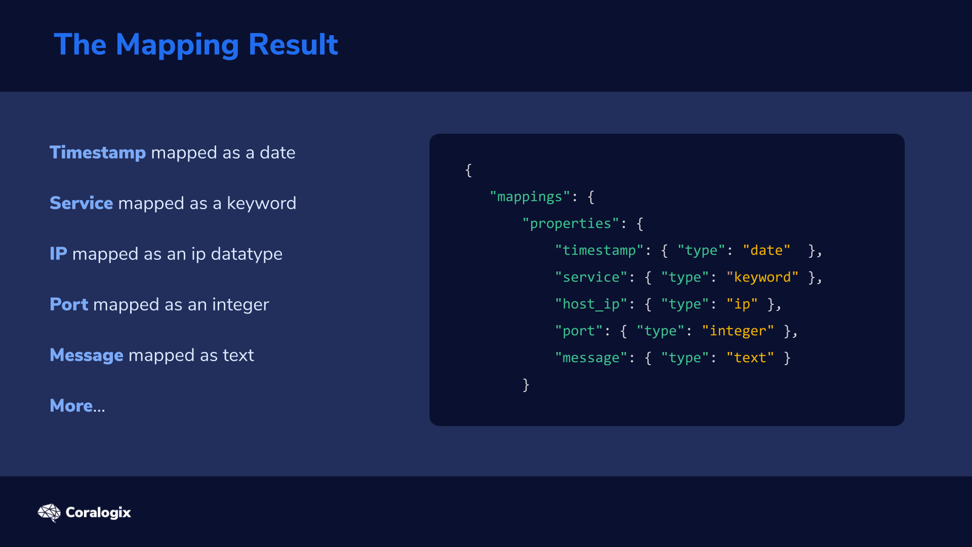


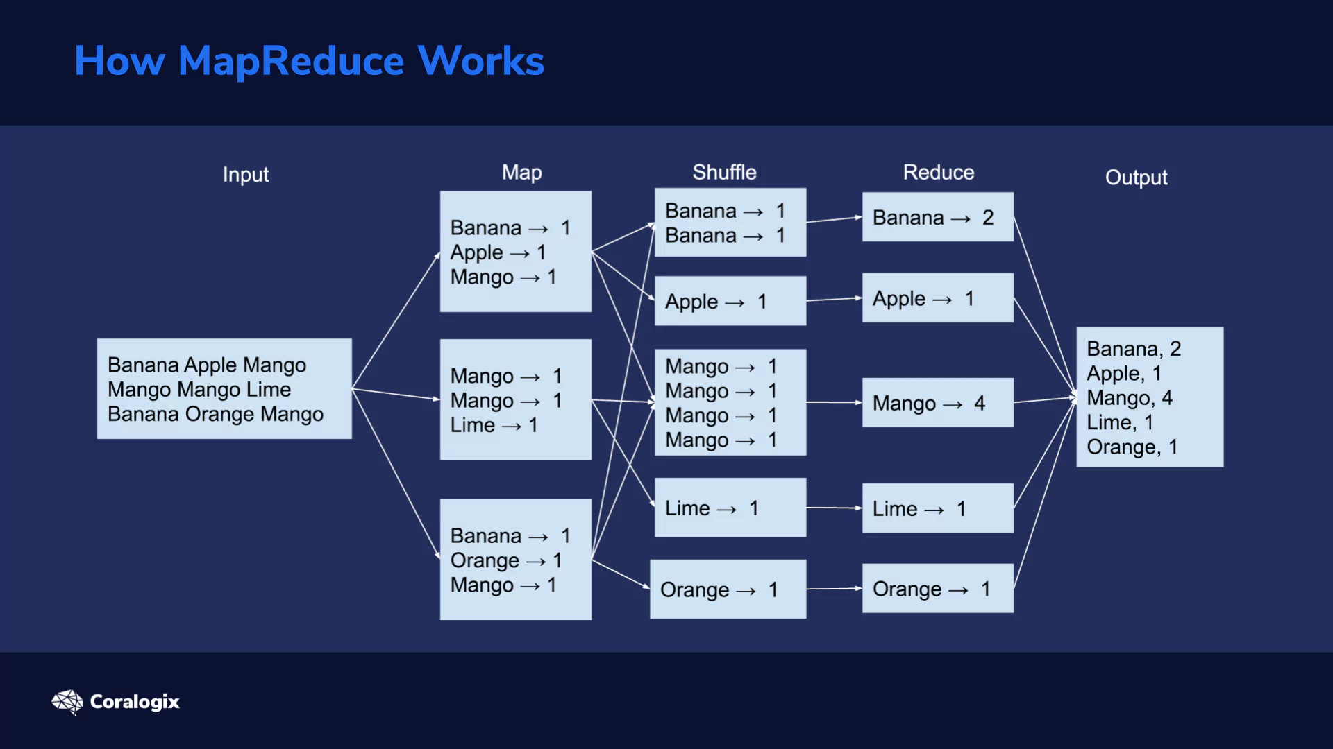
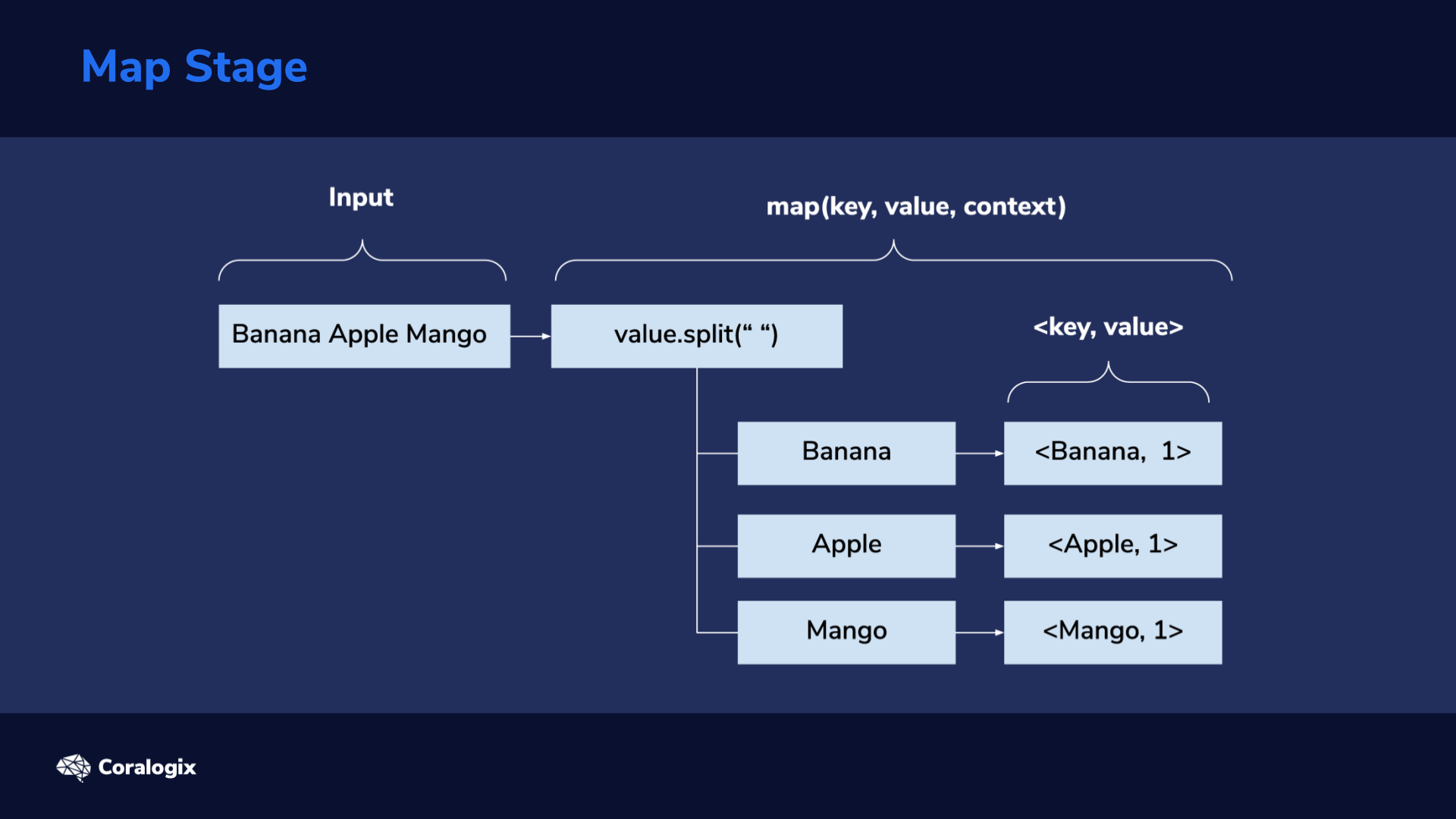
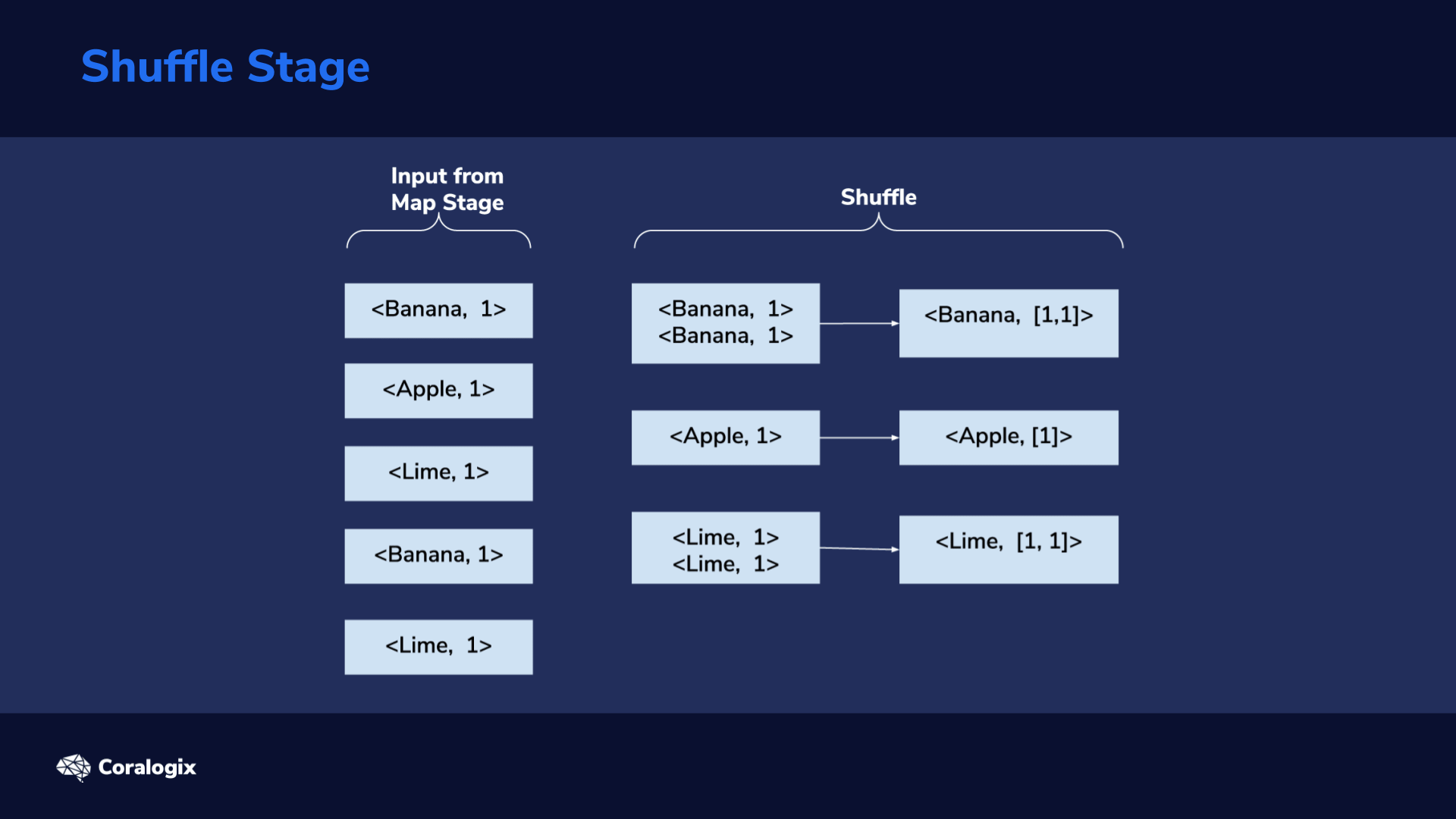
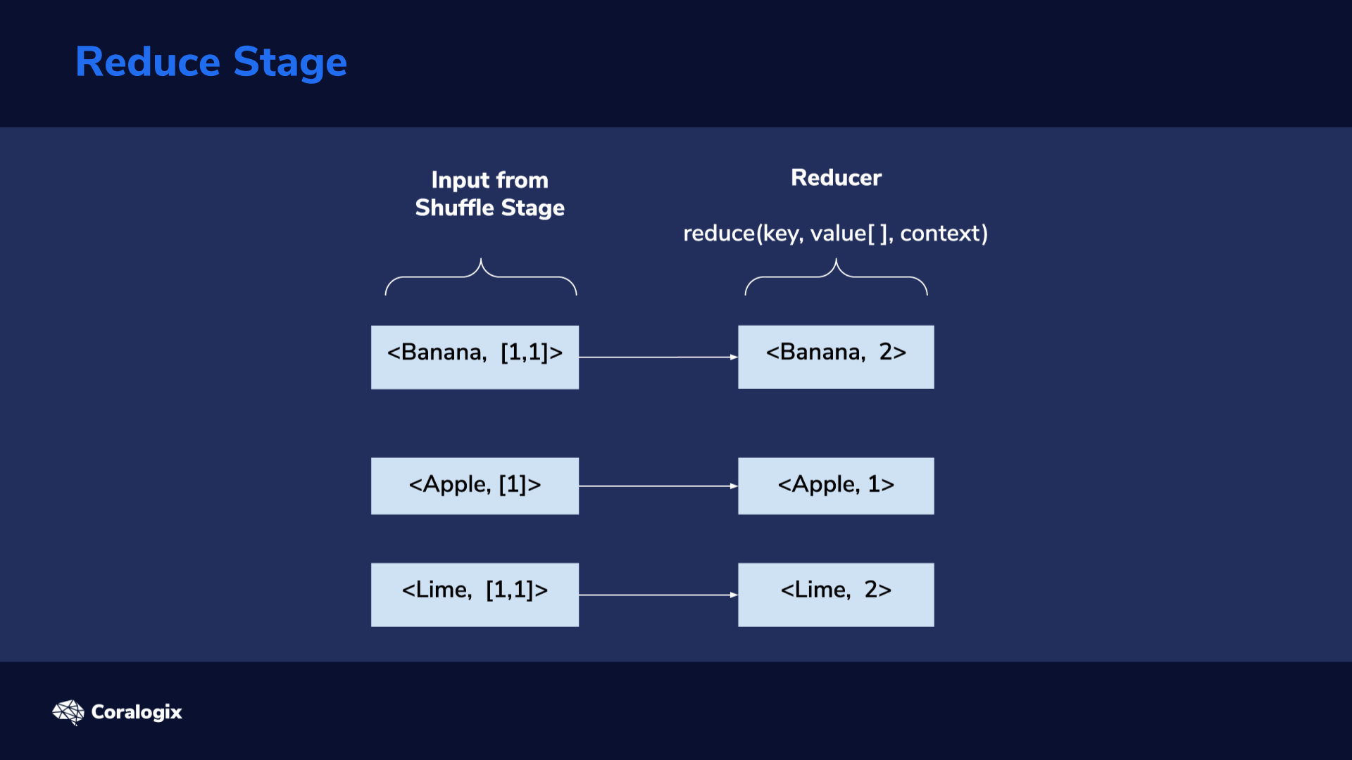
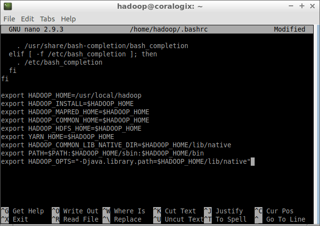
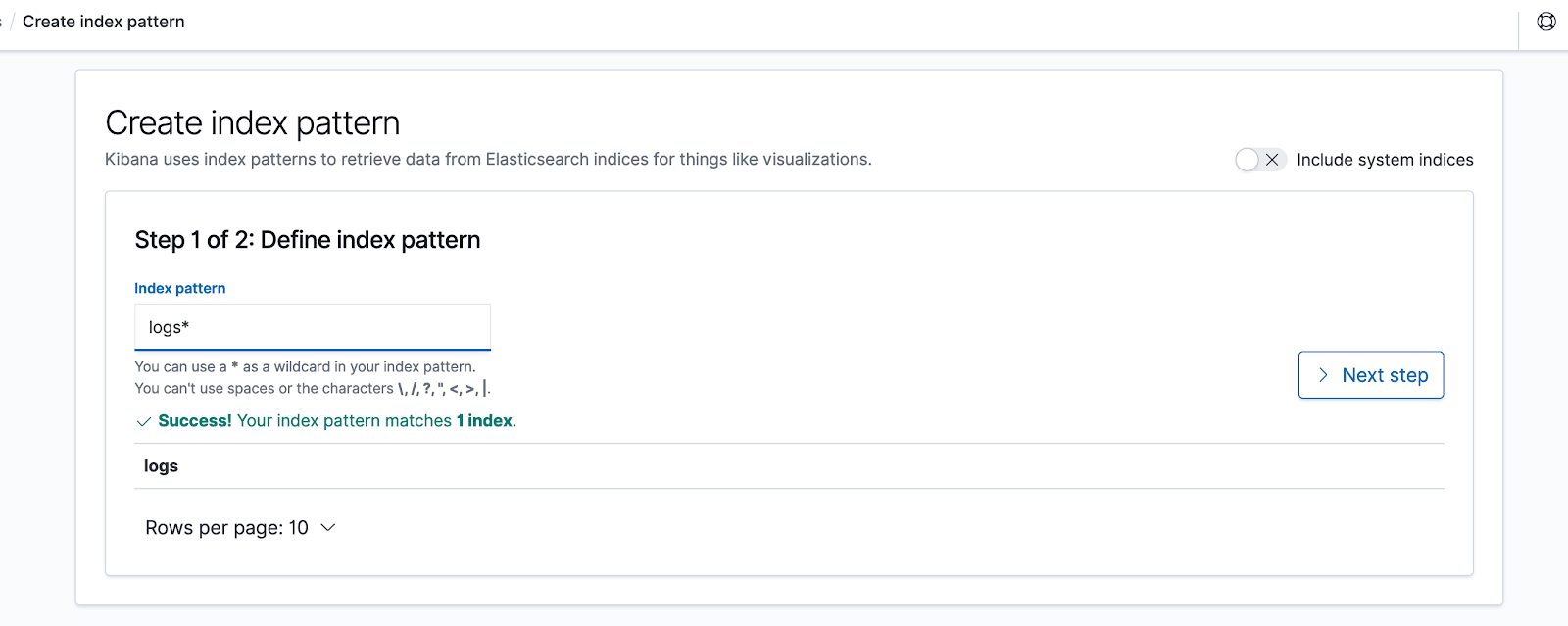
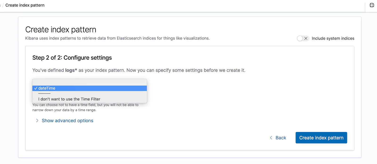
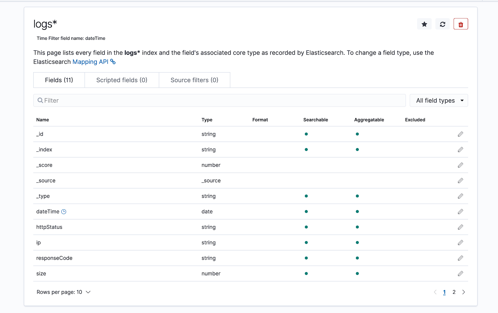
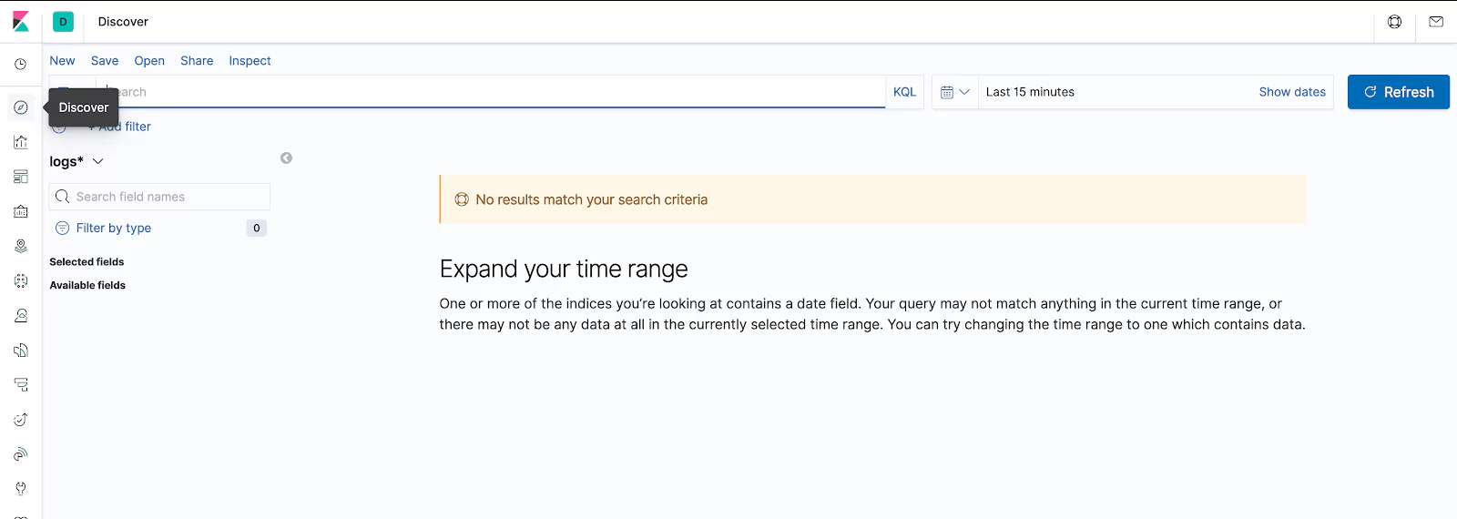
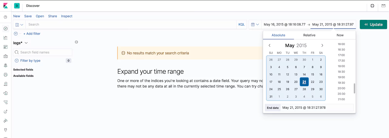
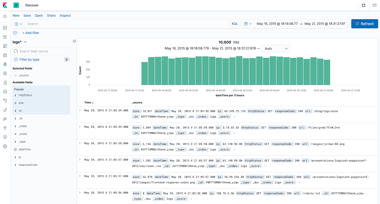
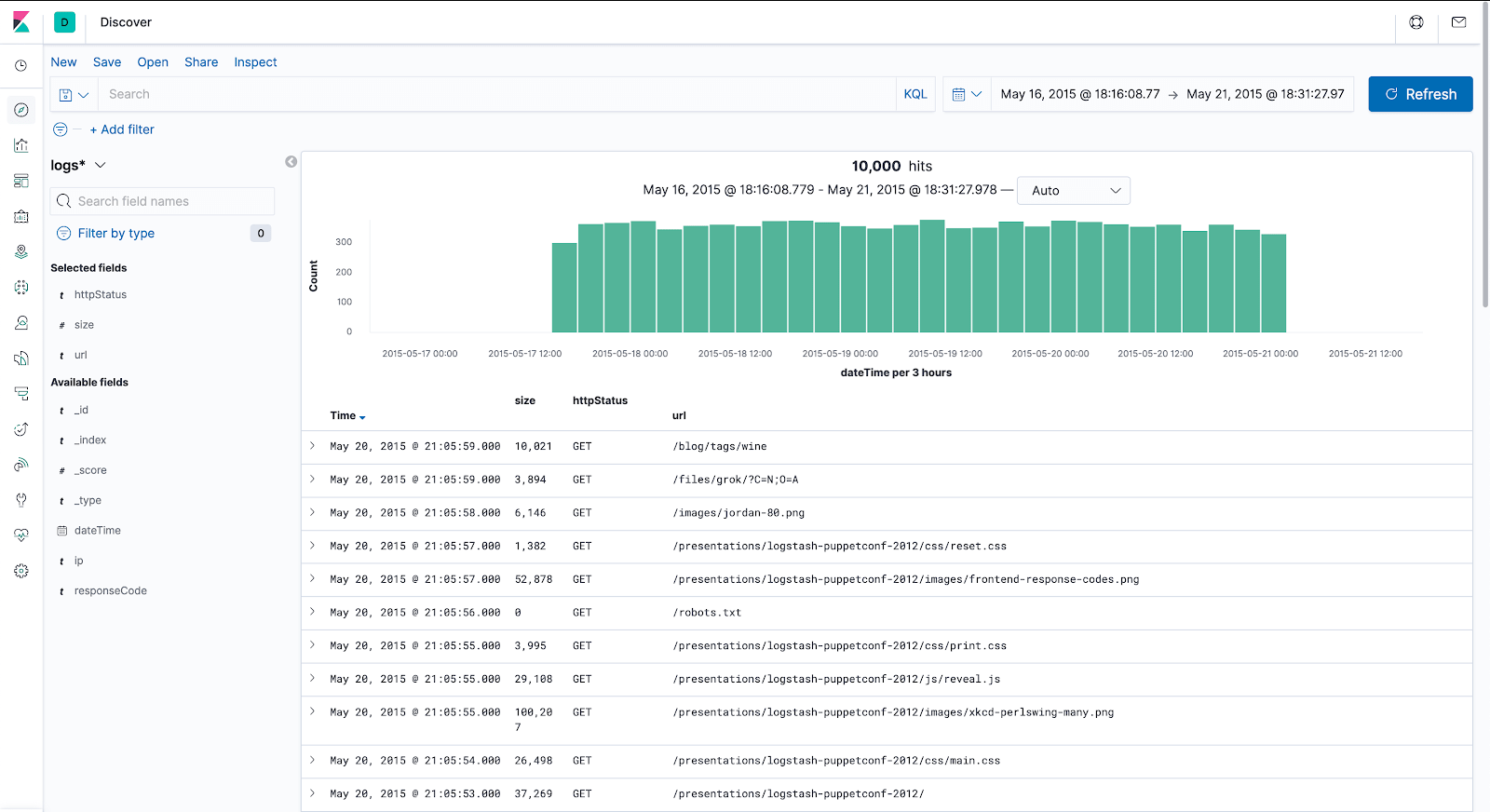
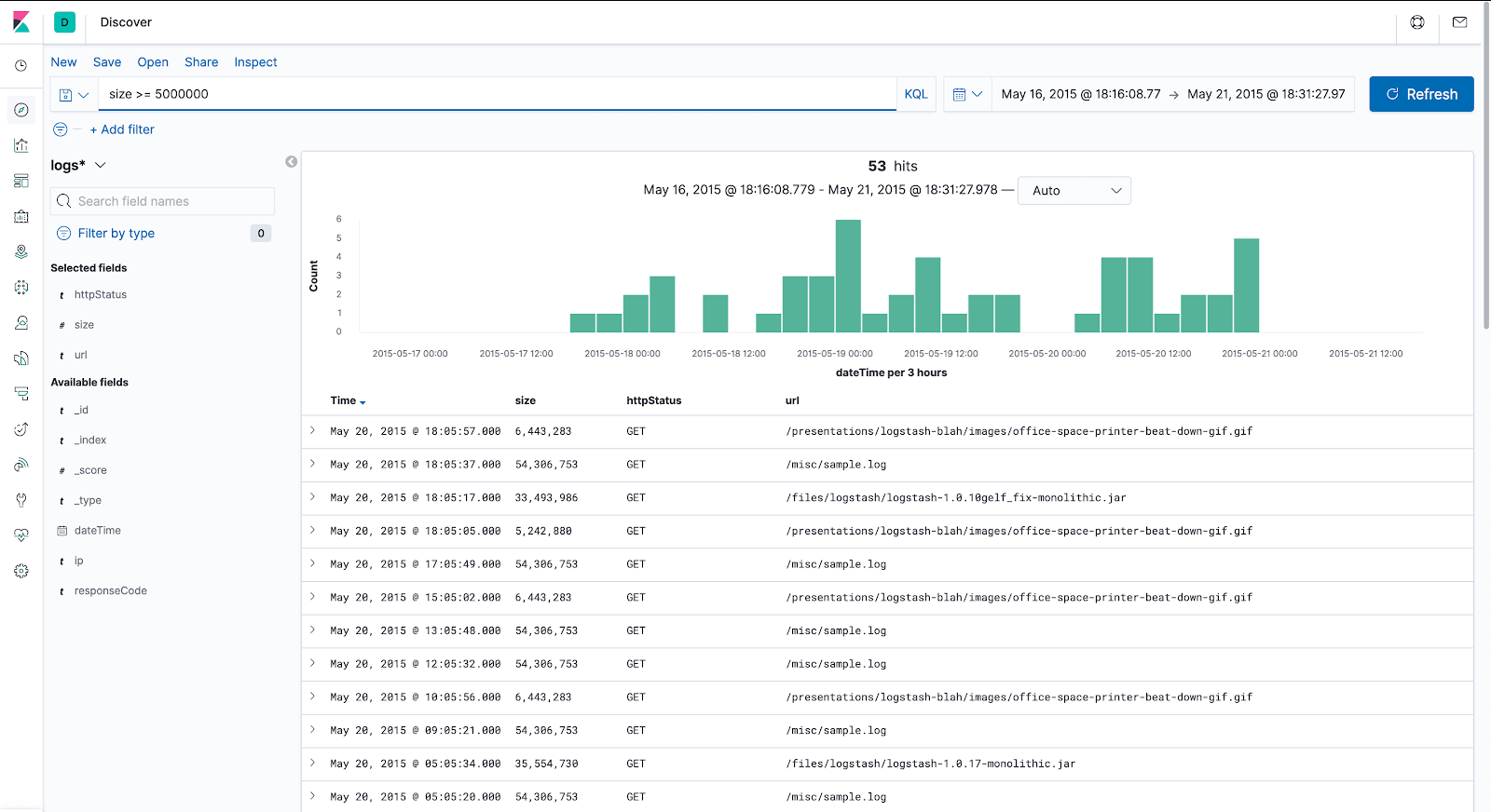
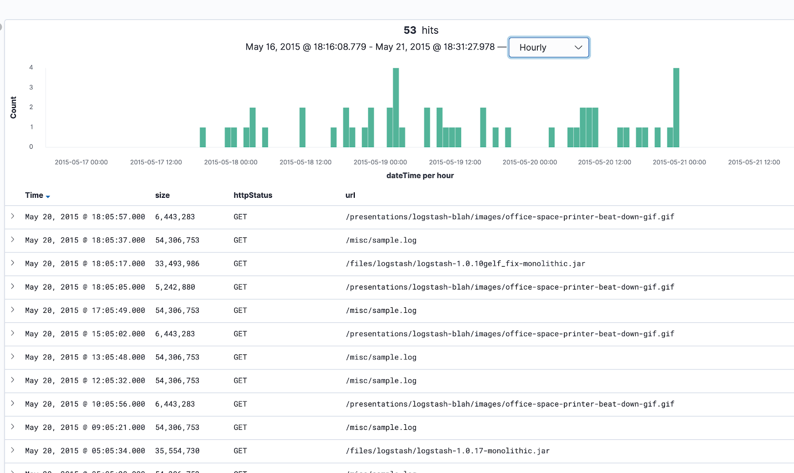

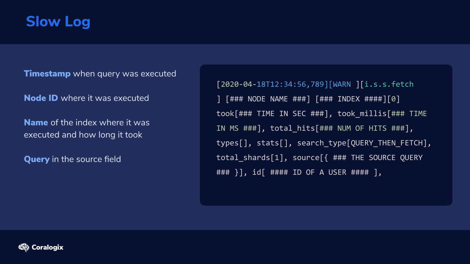
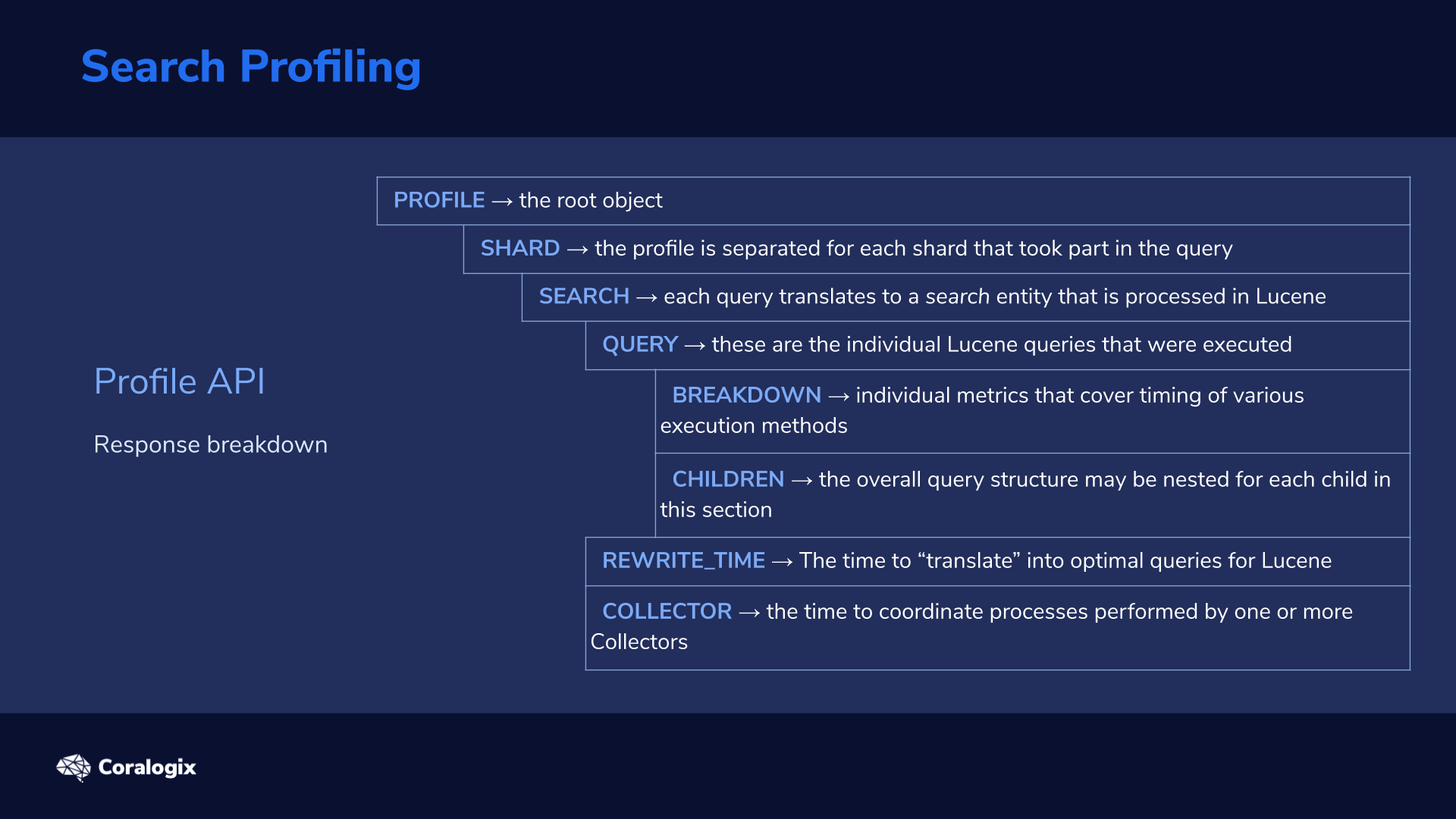
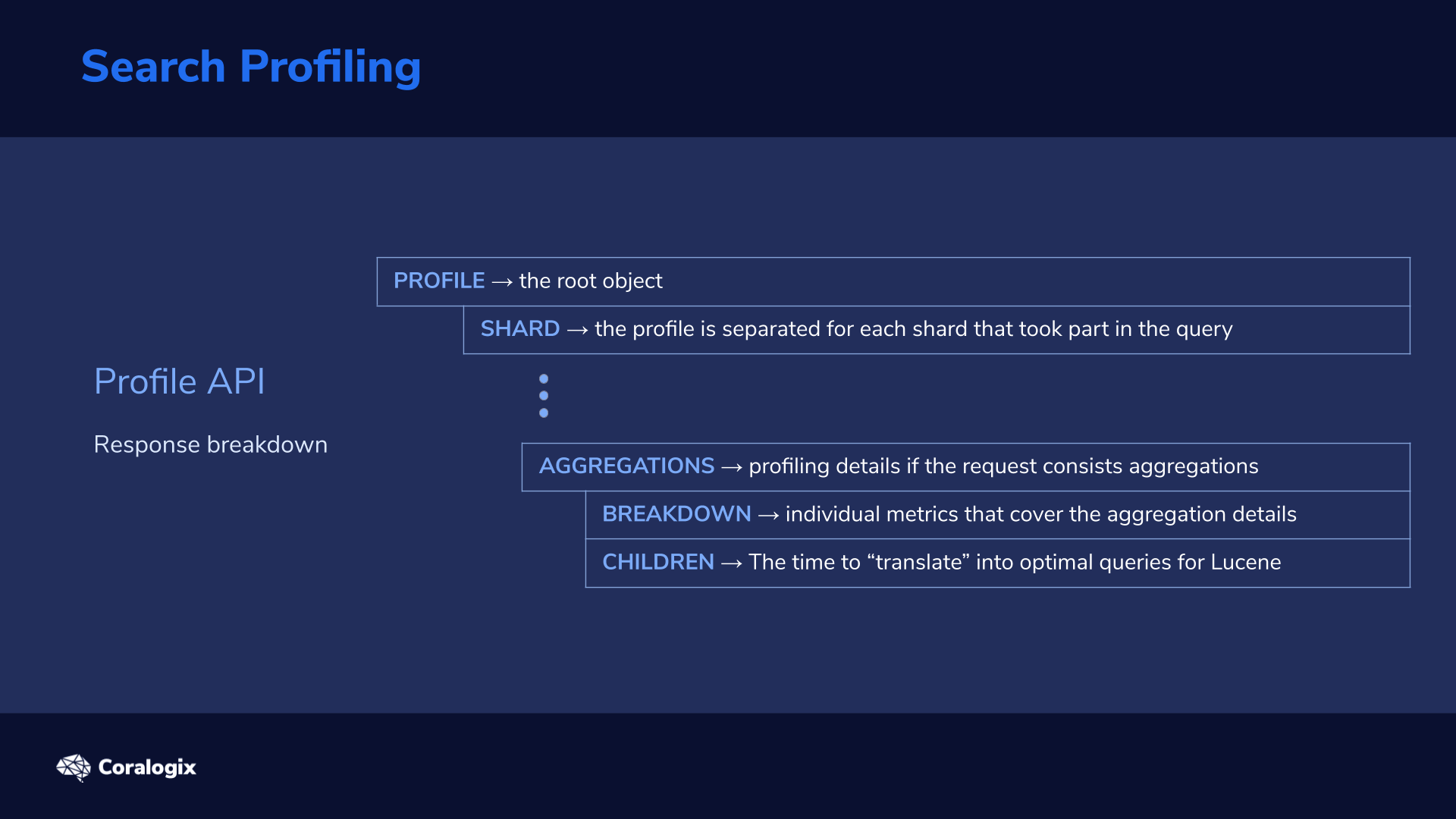
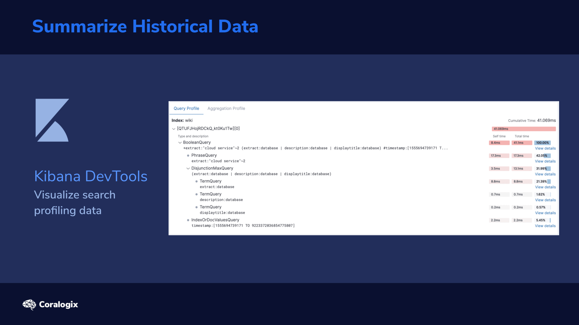
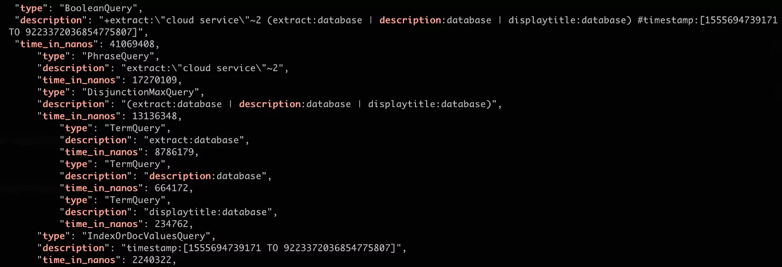

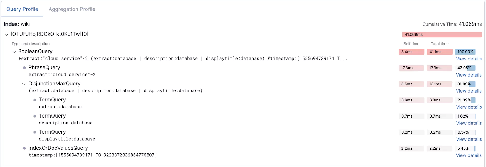

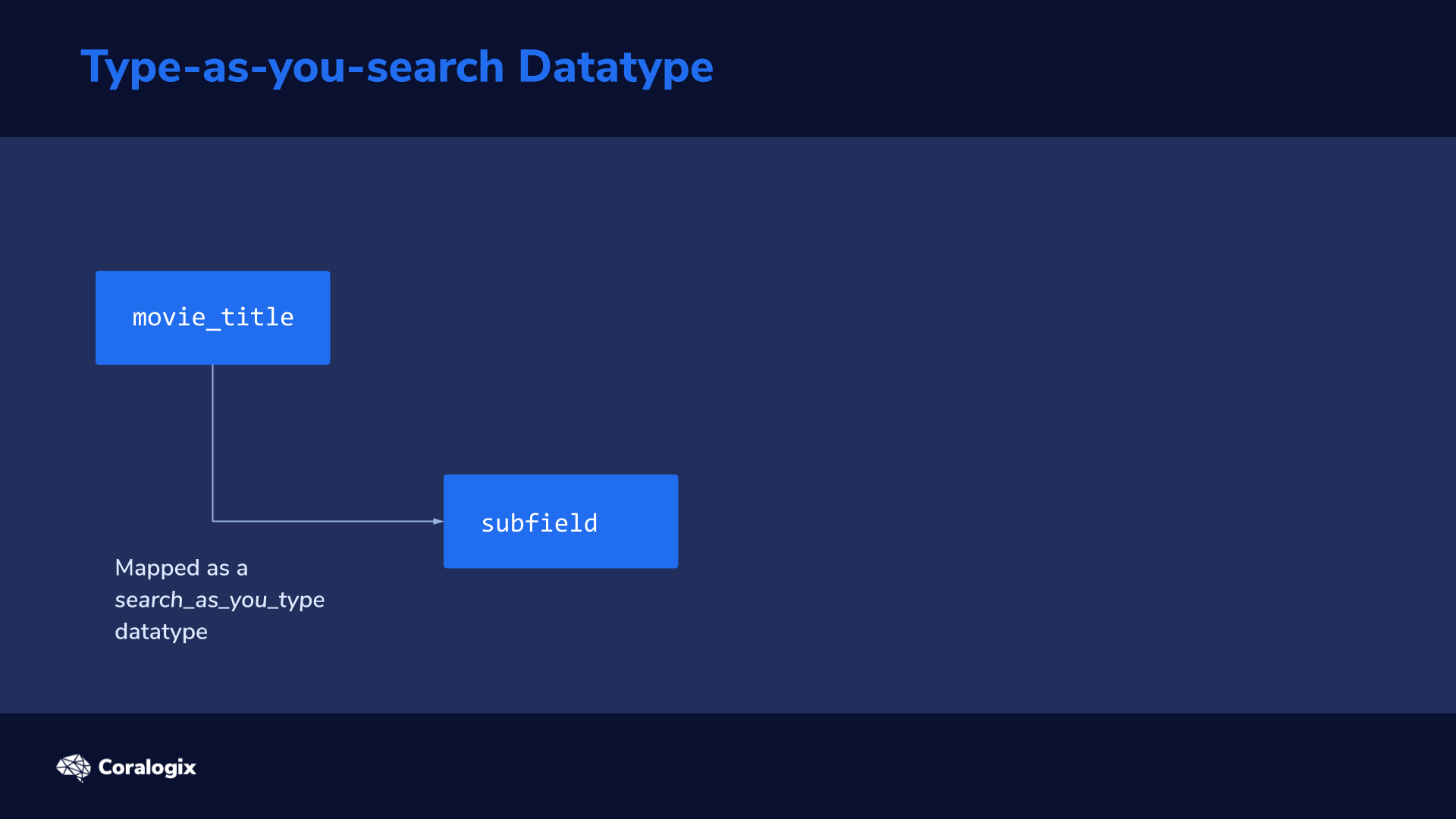
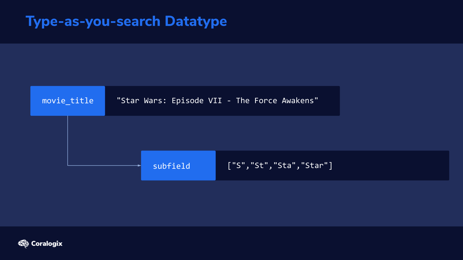
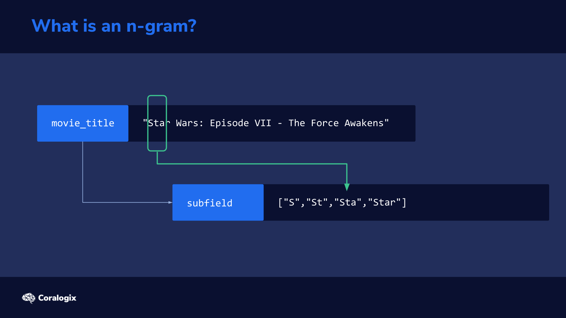
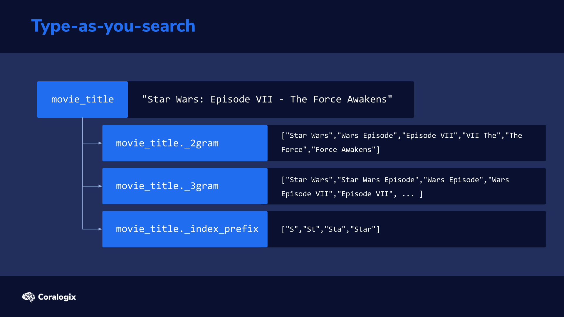


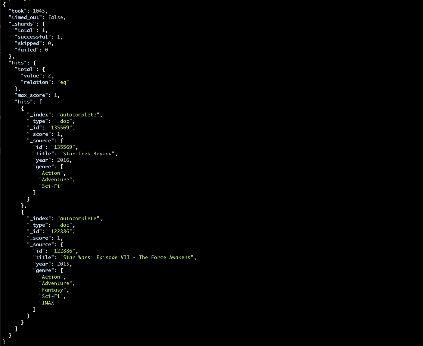


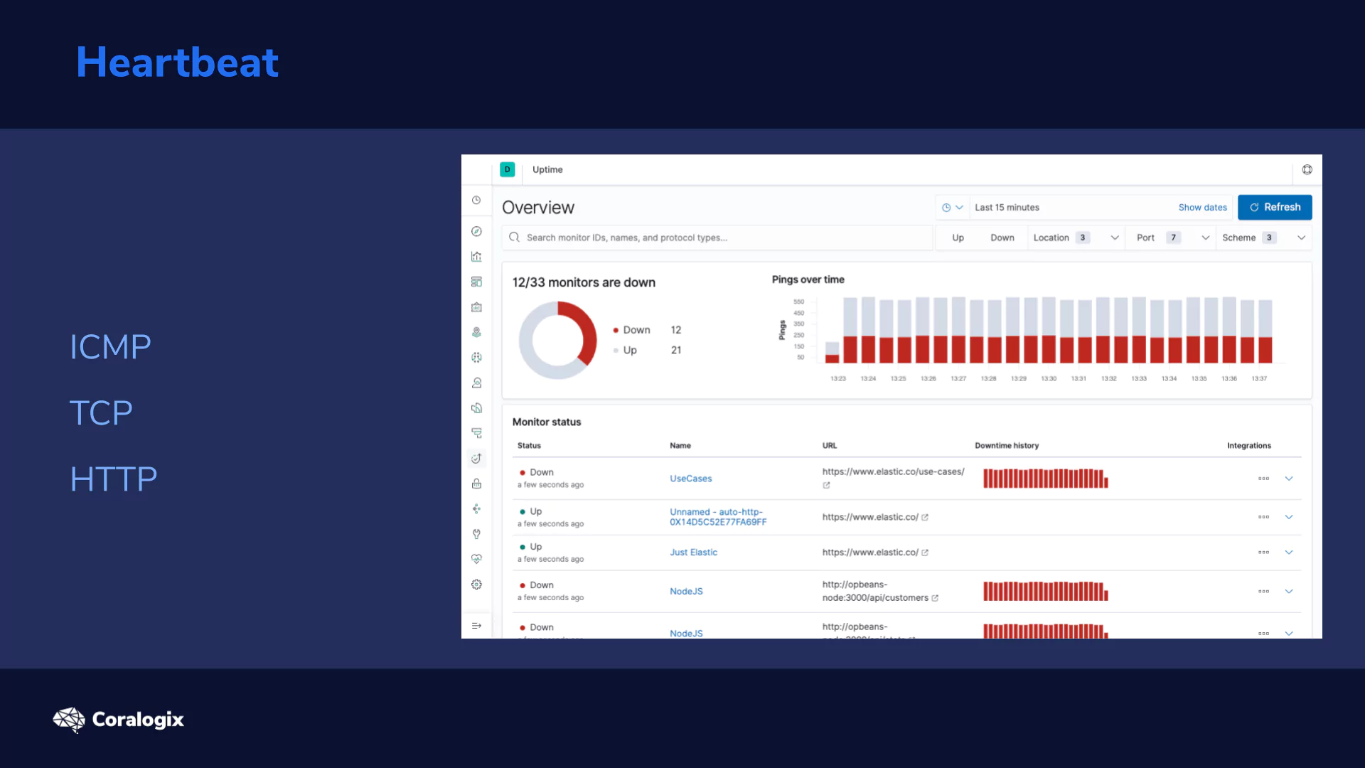


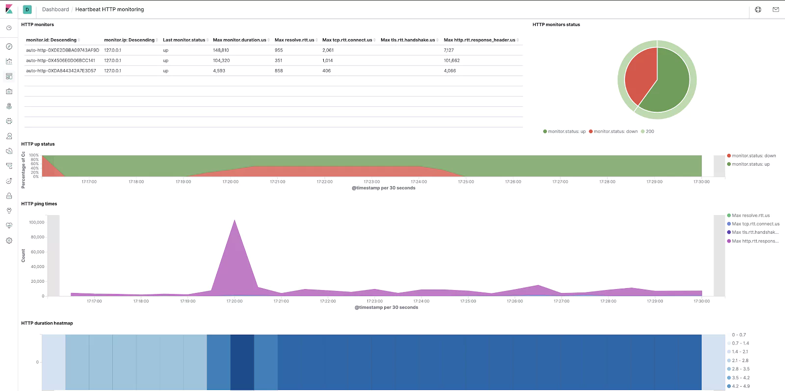

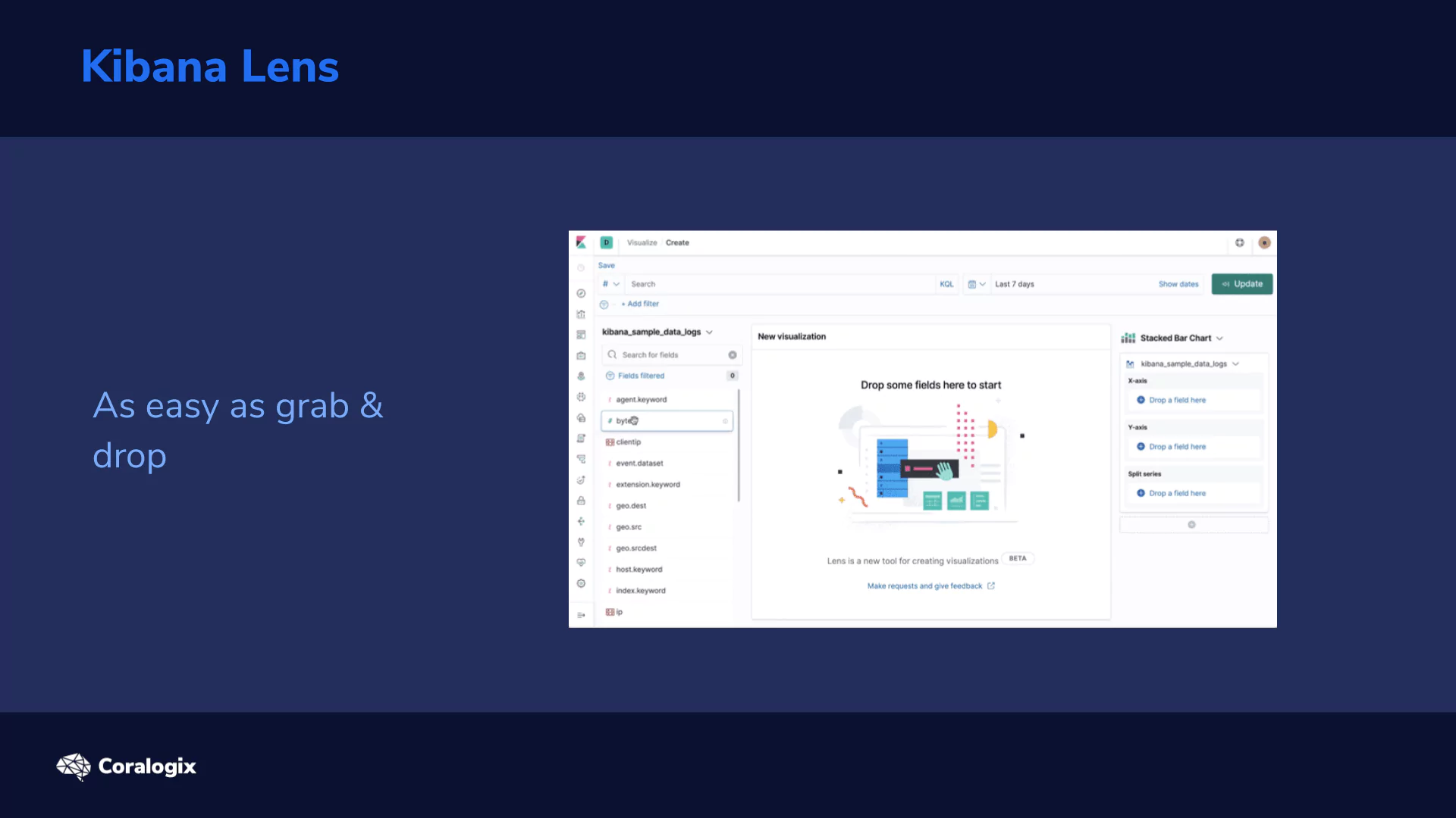
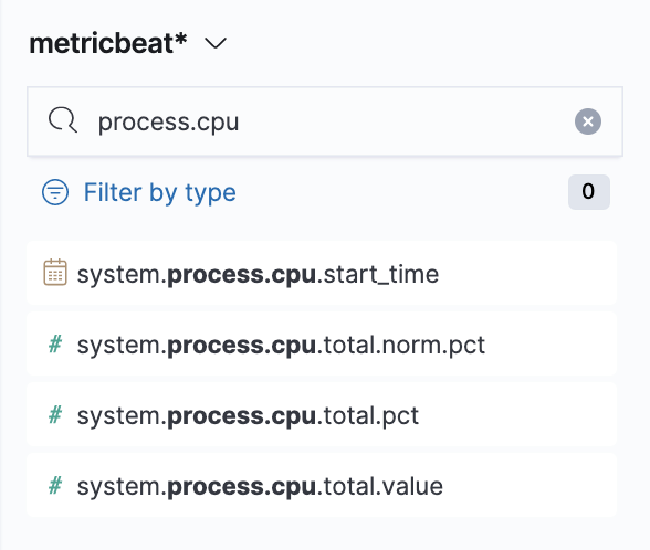
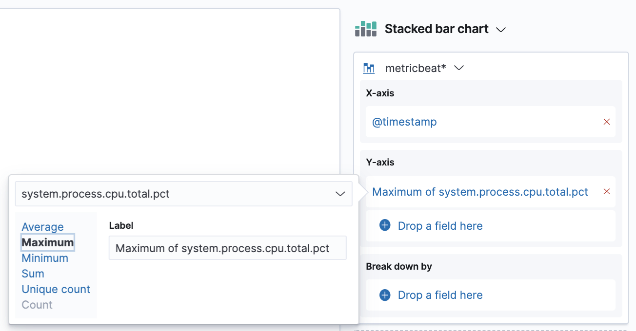
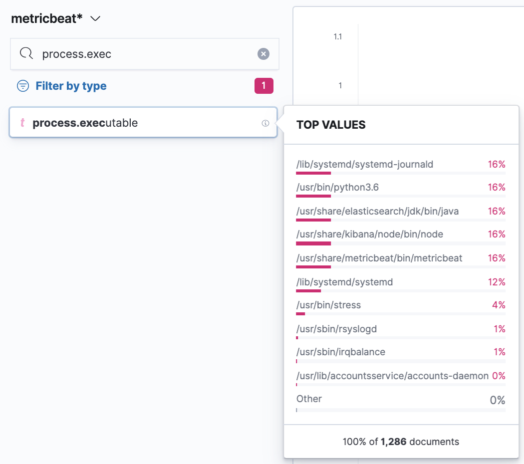
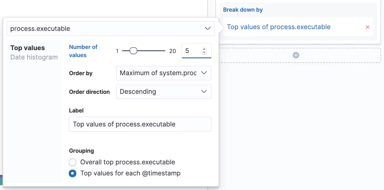
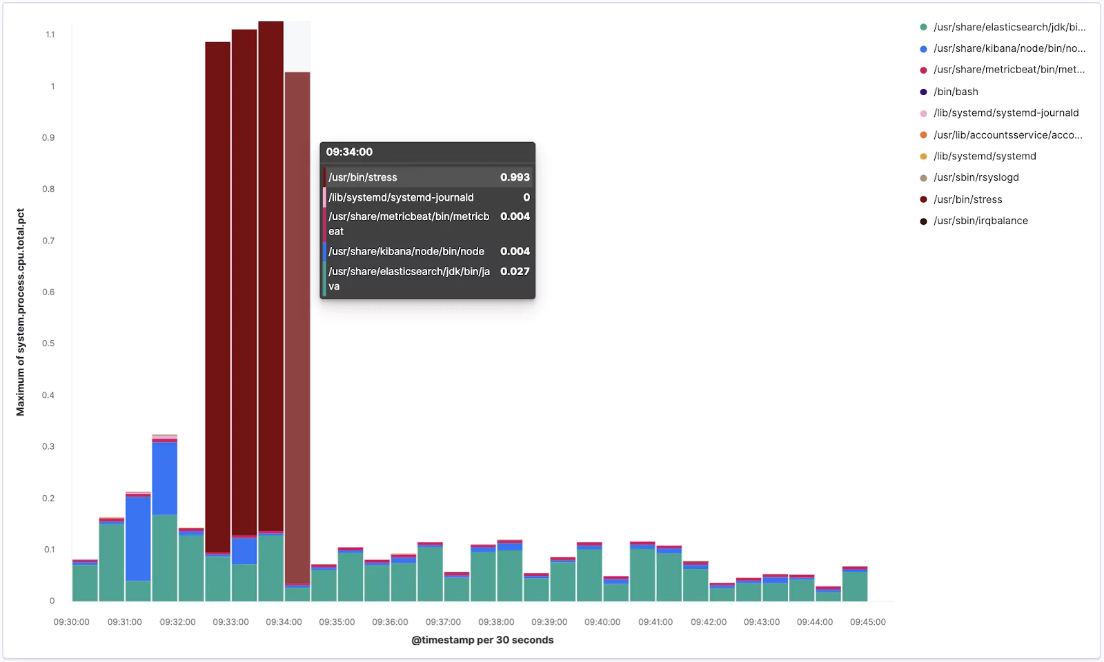
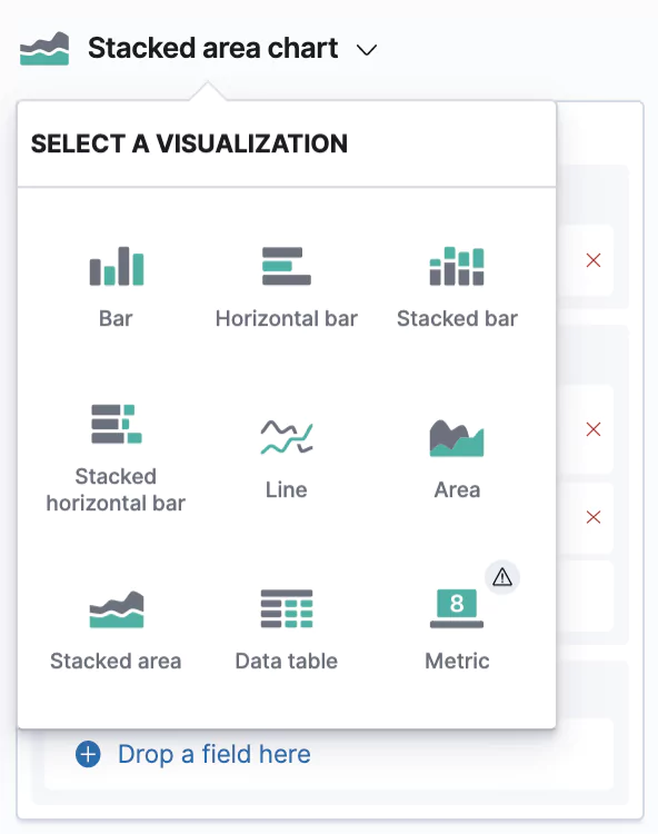
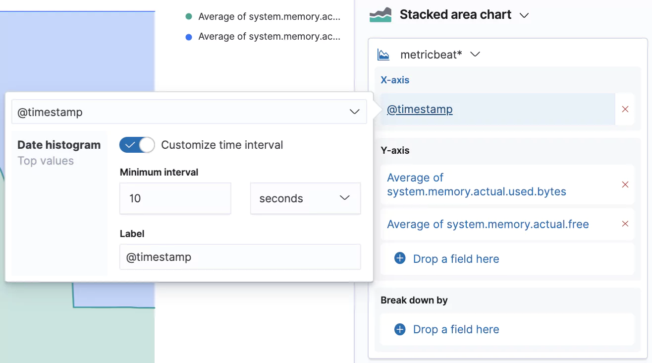
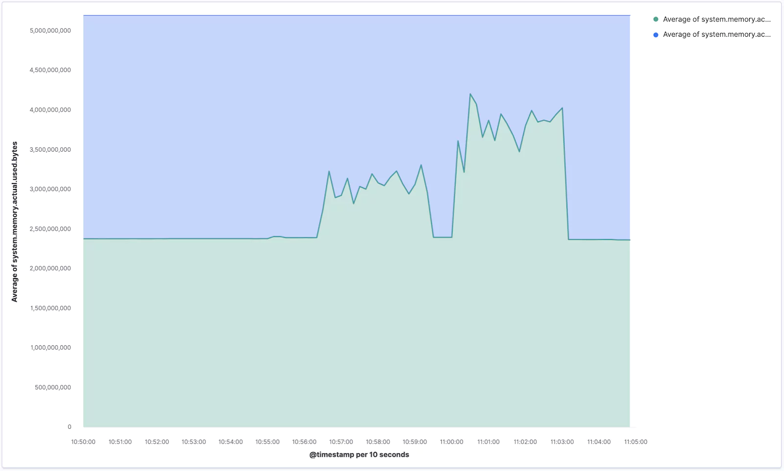


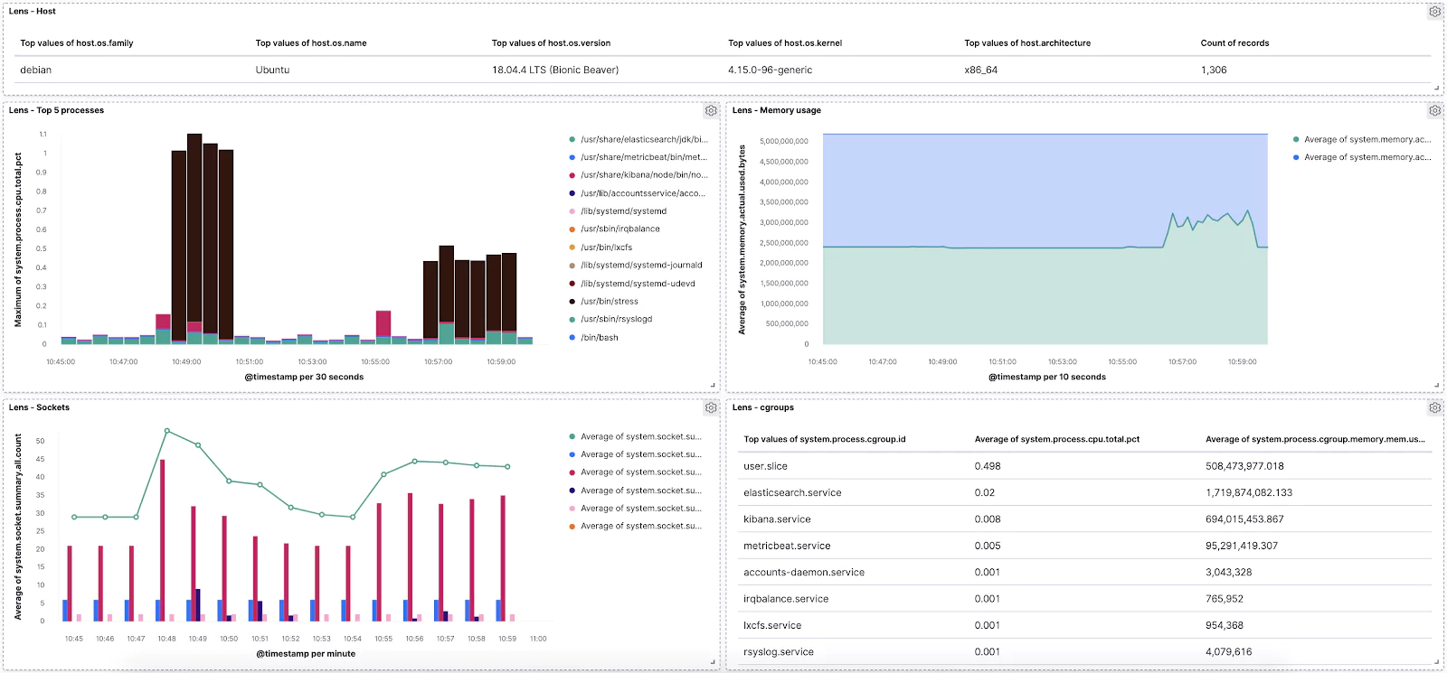

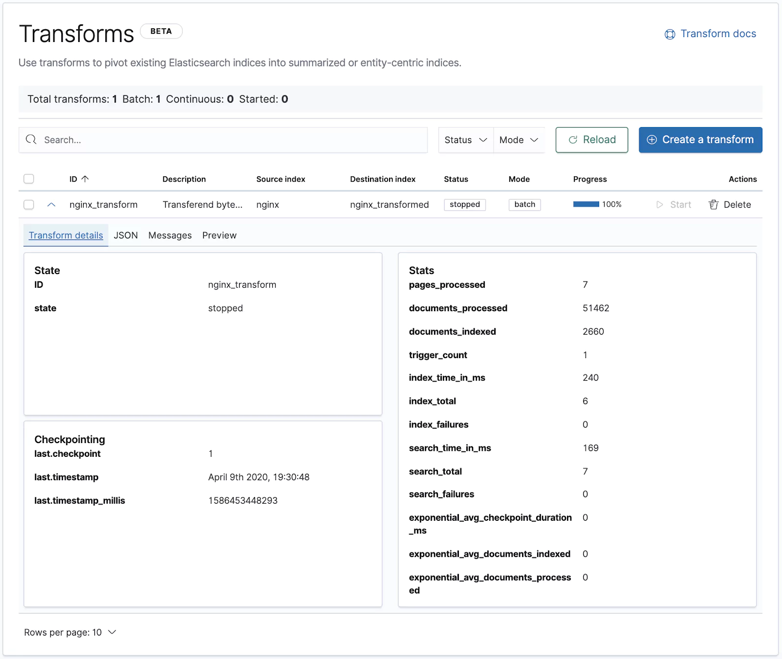
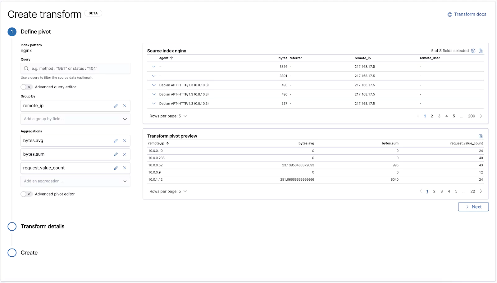
![Logstash CSV: Import & Parse Your Data [Hands-on Examples]](https://coralogix.com/wp-content/uploads/2025/06/42.png)
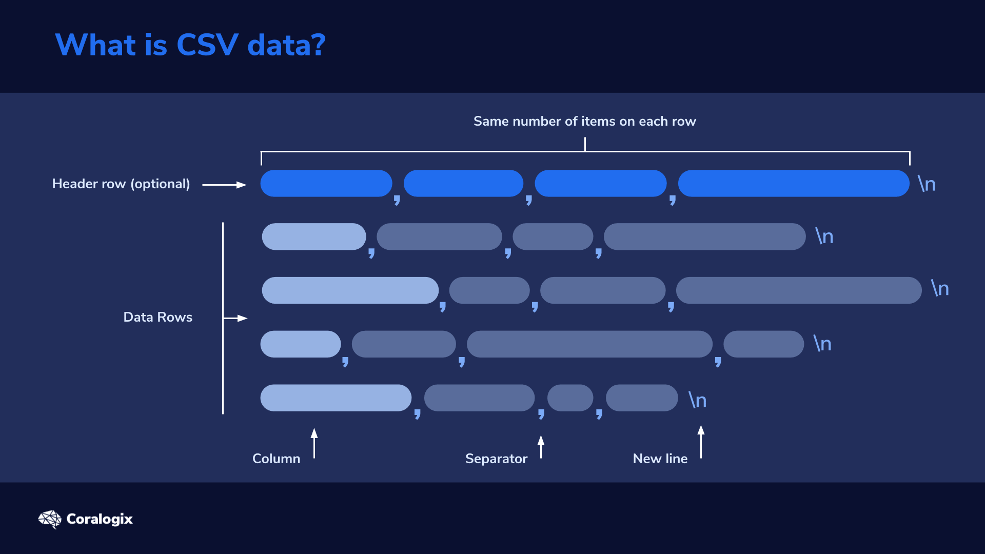
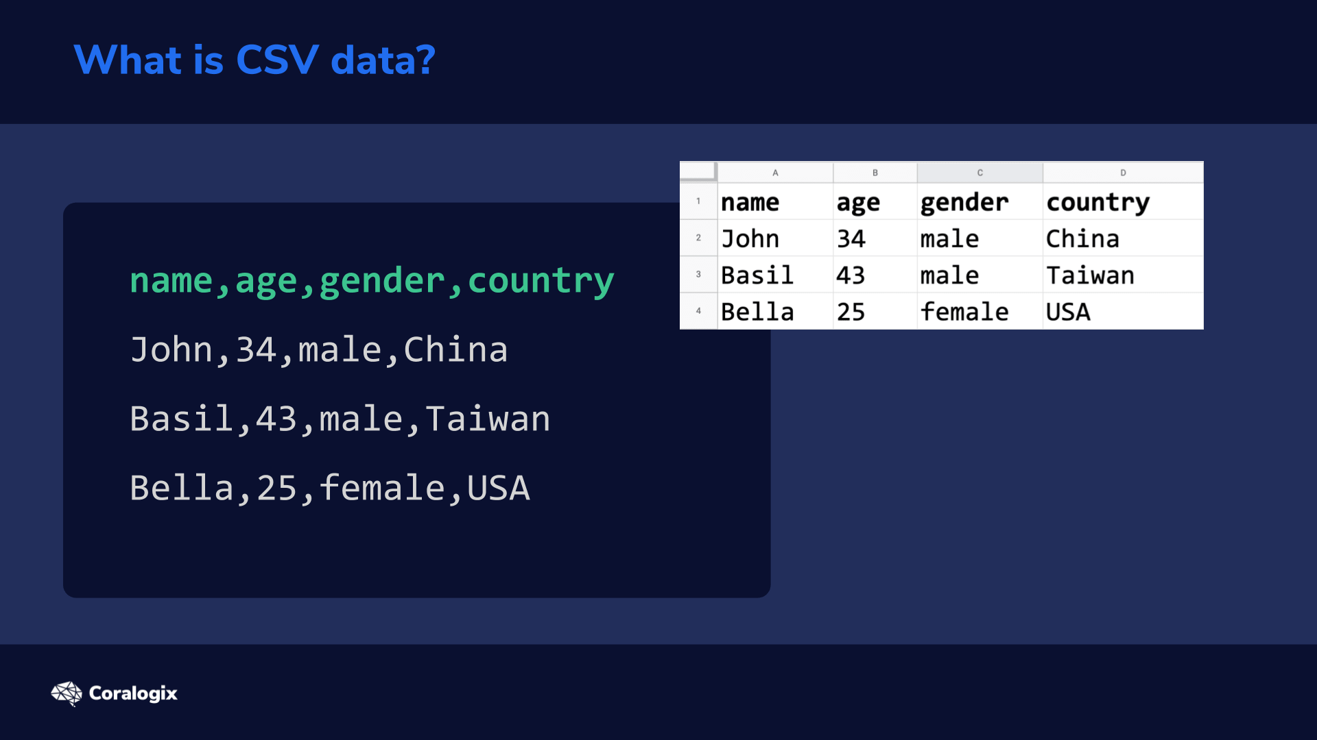
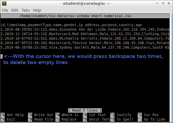
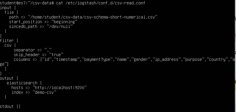
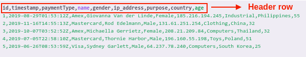
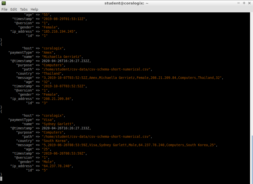
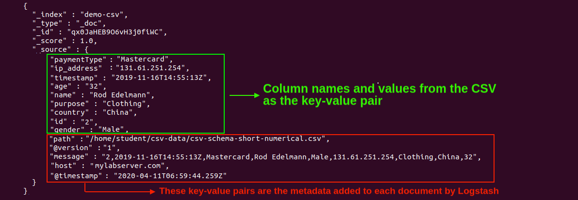
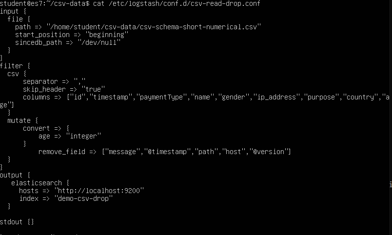

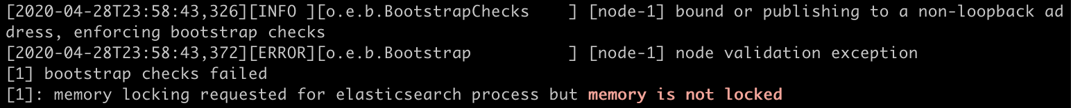


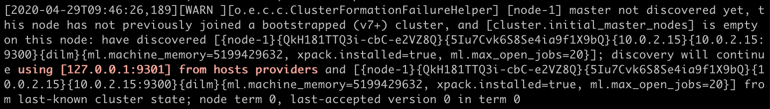
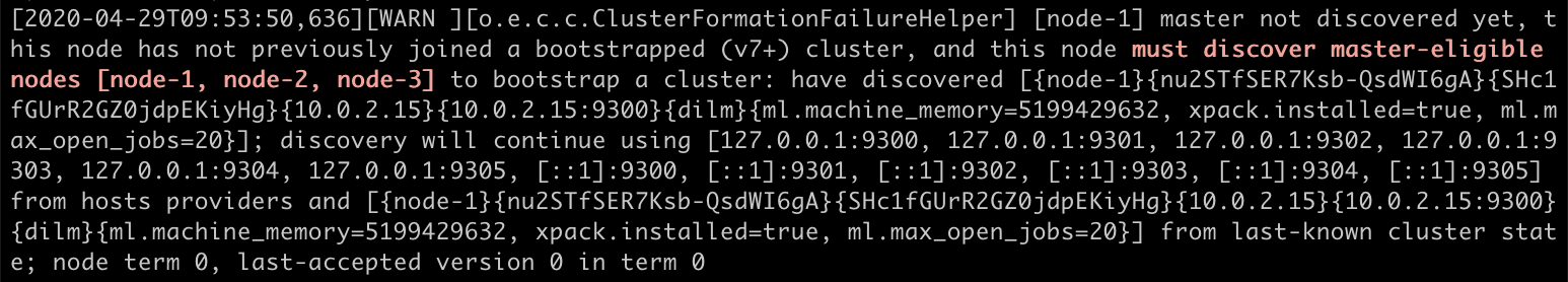

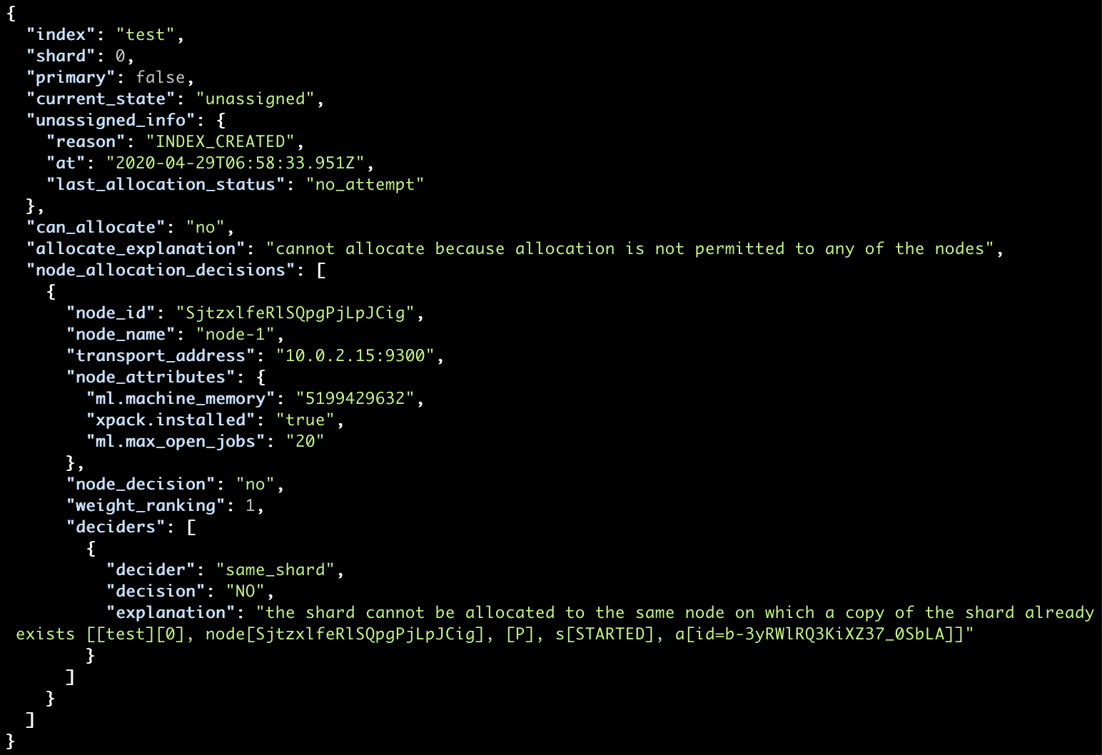

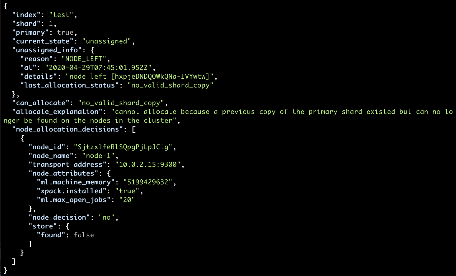
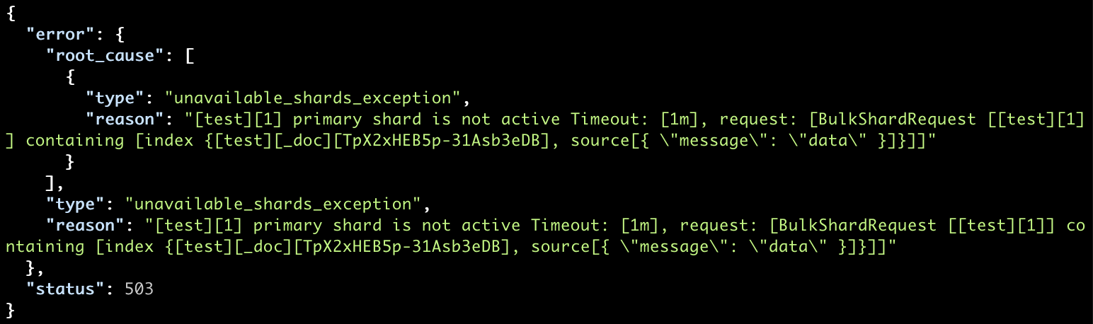

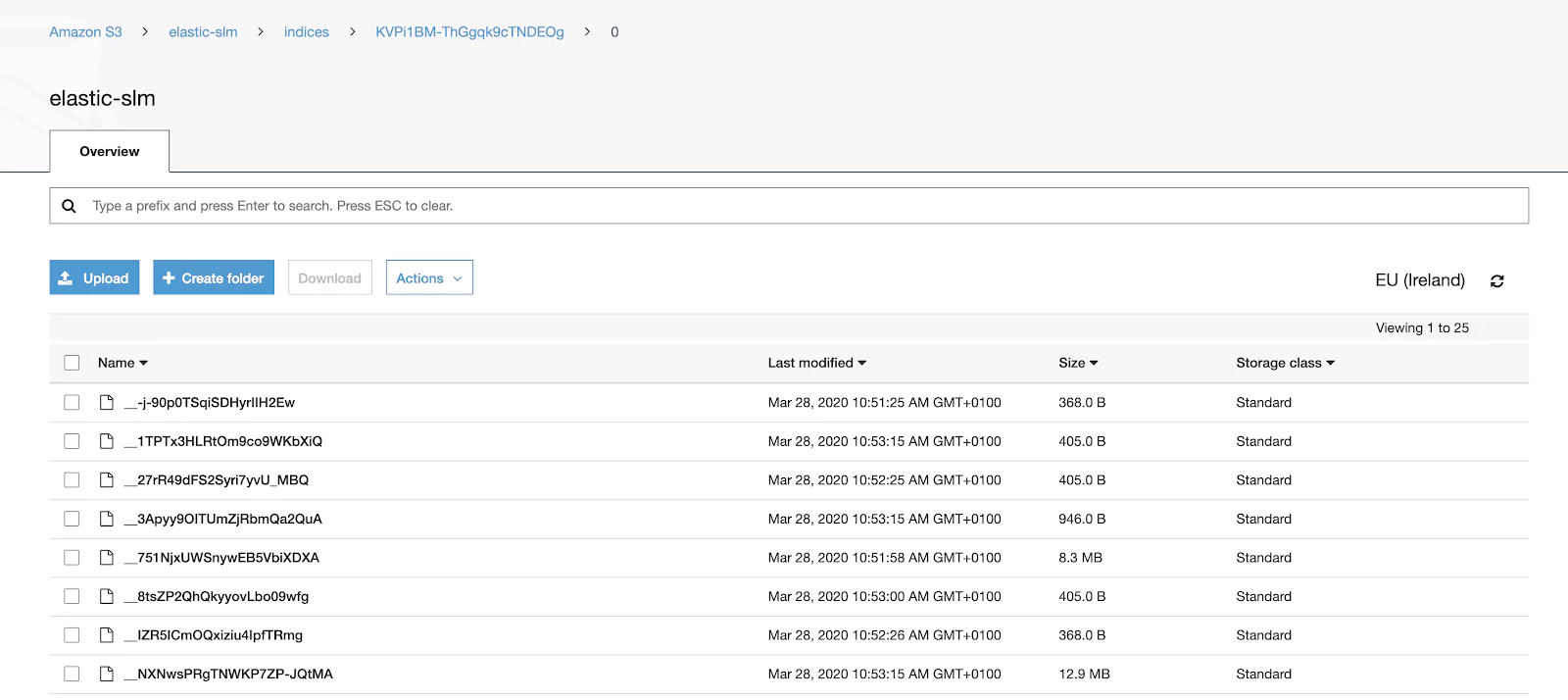

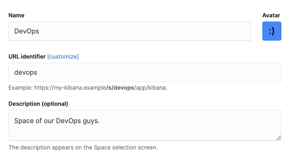
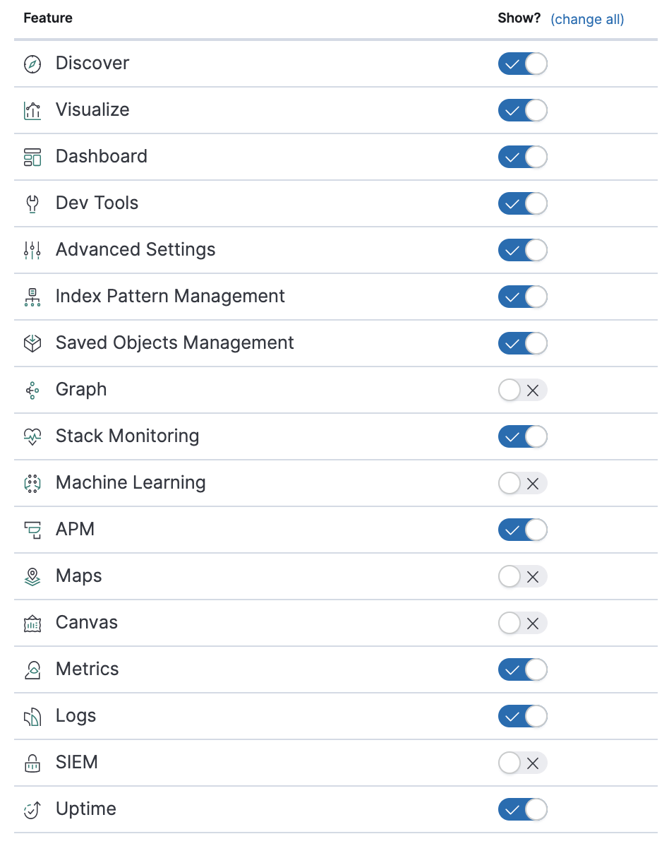
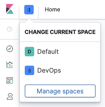
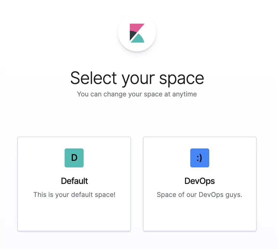

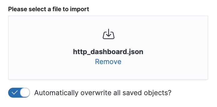
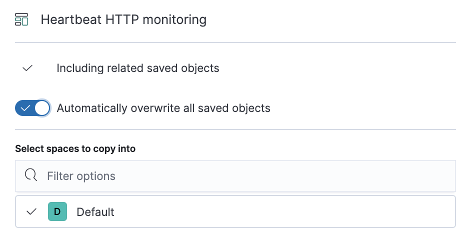
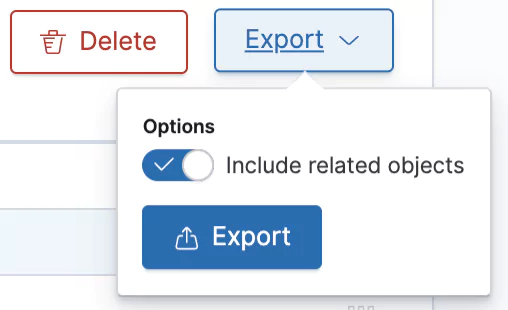


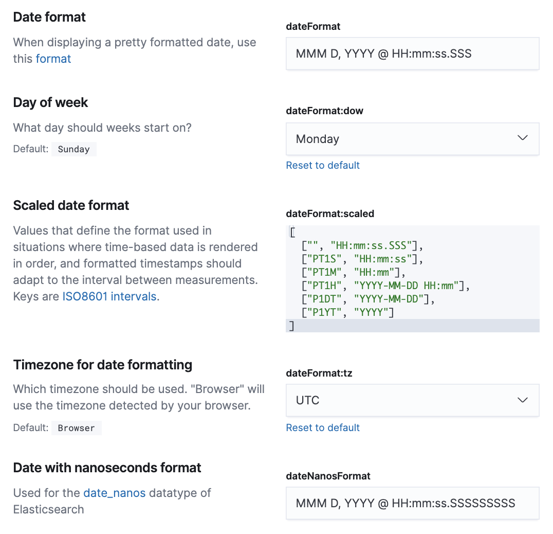

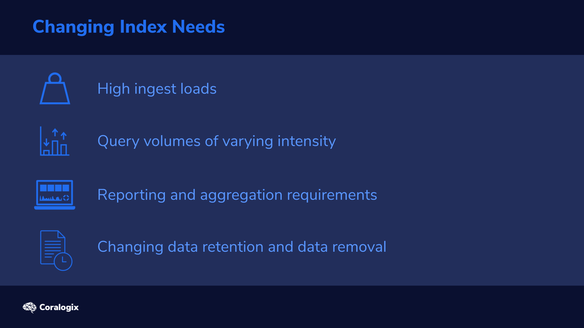
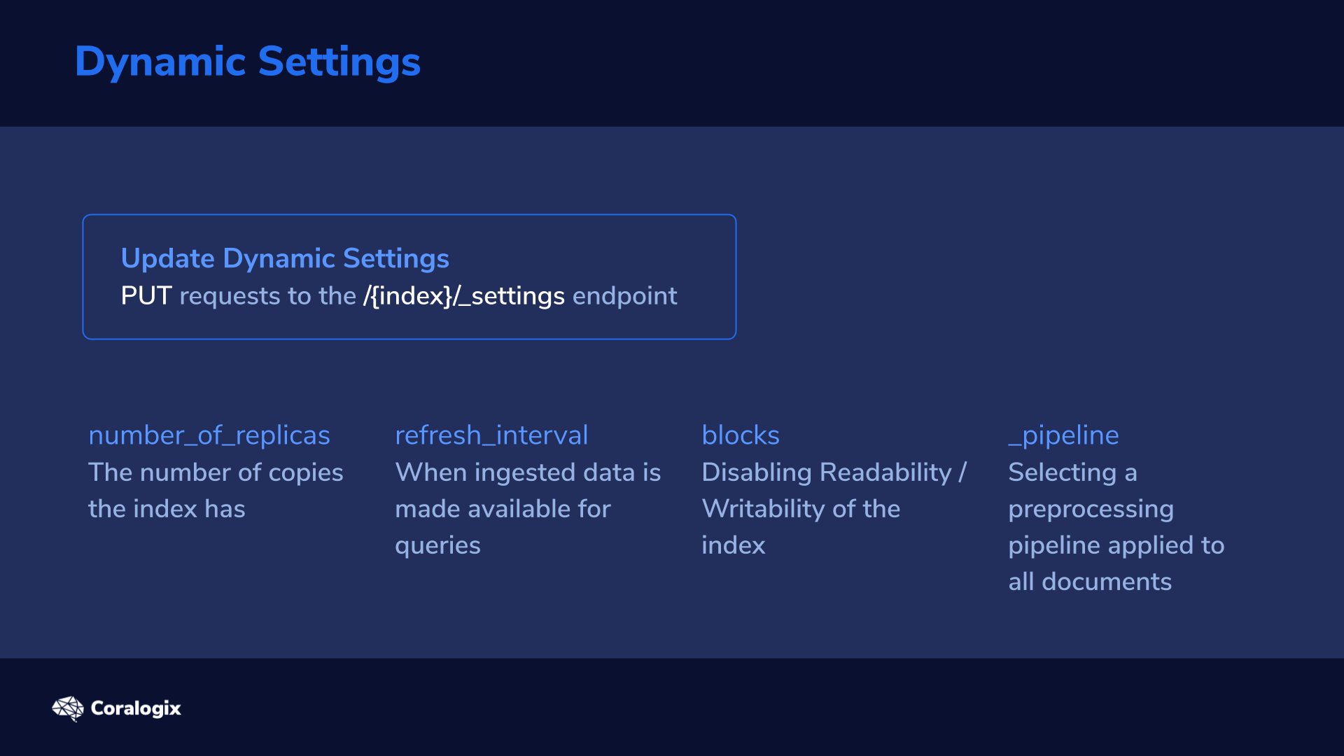
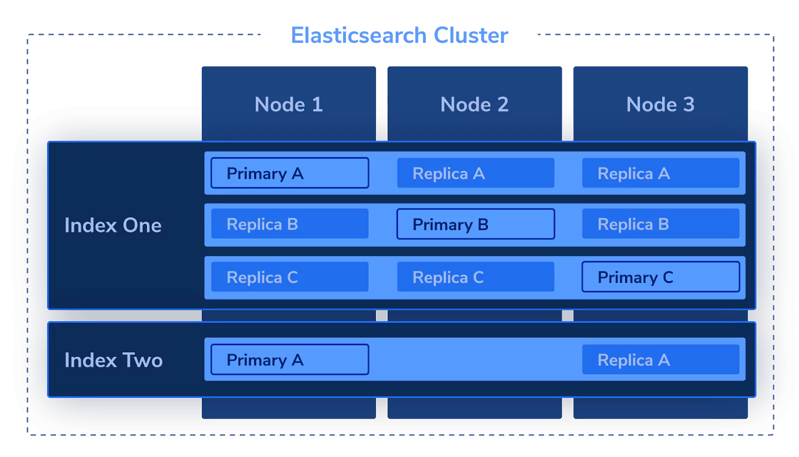
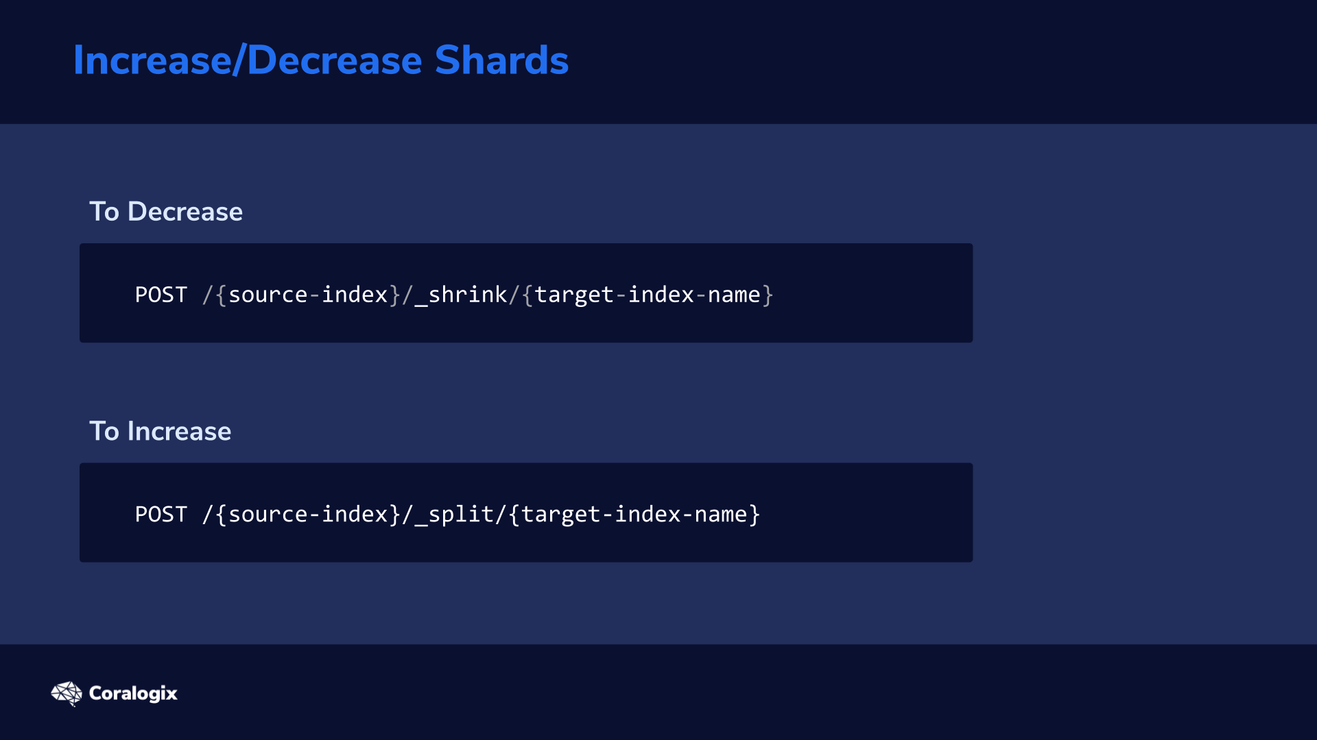

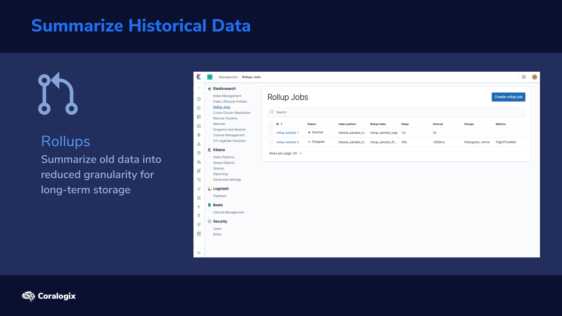

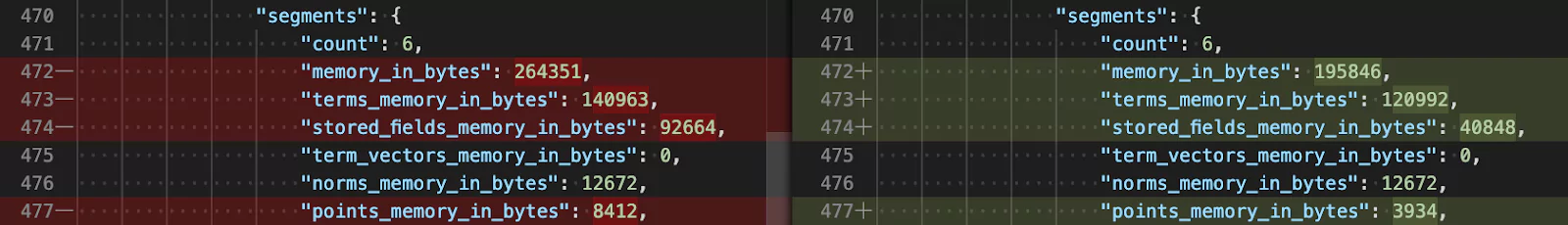
