Cloudwatch is the de facto method of consuming logs and metrics from your AWS infrastructure. The problem is, it is not the de facto method of capturing metrics for your applications. This creates two places where observability is stored, and can make it difficult to understand the true state of your system.
That’s why it has become common to unify all data into one place, and Prometheus offers an open-source, vendor-agnostic solution to that problem. But we need some way of integrating Cloudwatch and Prometheus together.
Why is one Observability source better than two?
Tool Sprawl is a real issue in the DevOps world. If your infrastructure metrics are held in one silo, and your application metrics are held elsewhere, what is the best way of correlating the two measurements? The truth is, it’s challenging to truly aggregate across multiple data sources. This is why, at Coralogix, we strongly advise that you aim for a single location to hold your telemetry data.
Fortunately, with Prometheus and Cloudwatch, there is the perfect tool in existence.
The Prometheus Cloudwatch Exporter
To ingest Cloudwatch metrics into Prometheus, you will need to use a tool called the Prometheus Cloudwatch Exporter. This tool is a Prometheus exporter that runs on Amazon Linux, and it allows you to scrape metrics from Cloudwatch and make them available to Prometheus.
This tool acts as the bridge between Cloudwatch and Prometheus. It will unify all your application and infrastructure metrics into a single repository, which can be correlated and analyzed.
Prerequisites
You’ll need a running Amazon EC2 instance. This can be part of a Kubernetes cluster, but we’re keeping things simple for this tutorial.
Once your EC2 instance is running, you will need to install the Prometheus Cloudwatch Exporter. You can do this by running the following command from the terminal:
After downloading the Prometheus Cloudwatch Exporter, you will need to unpack the binary and make it executable. You can do this by running the following commands:
tar -xf cloudwatch_exporter-*.tar.gzcd cloudwatch_exporter-*chmod +x cloudwatch_exporter
Once the Prometheus Cloudwatch Exporter is installed, you will need to configure it to scrape your Cloudwatch metrics. You can create a new configuration file and specify the metrics you want to scrape. Here is an example configuration file:
After you have created your configuration file, you can start the Prometheus Cloudwatch Exporter by running the following command:
./cloudwatch_exporter -config.file=config.yml
Finally, you will need to configure Prometheus to scrape the metrics from the Prometheus Cloudwatch Exporter. You can do this by adding the following configuration to your Prometheus configuration file:
Once you have completed these steps, Prometheus should start scraping metrics from Cloudwatch and making them available for you to query.
Does this sound like a lot of work?
It is – managing all of your own observability data can be painful. Rather than do it all yourself, why not check out the Coralogix documentation, which shows various options for integrating Coralogix and Cloudwatch. With massive scalability, a uniquely powerful architecture, and some of the most sophisticated observability features on the market, Coralogix can meet and beat your demands!
With dozens of microservices running on multiple production regions, getting to a point where any error log can be immediately identified and resolved feels like a distant dream. As an observability company, we at Coralogix are pedantic when it comes to any issue in one of our environments.
That’s why we are using an internal Coralogix account to monitor our development and production environments.
After experiencing a painful issue a few weeks ago, we started the process of adopting a zero-error policy on our team.
What is a Zero-Error Policy?
Preston de Guise first laid out his definition for a zero-error policy back in 2009 for data backups and protection. The policy soon gained popularity as a strategy for maintaining quality and reliability across all systems.
The three fundamental rules that de Guise lays out are:
All errors shall be known
All errors shall be resolved
No error shall be allowed to continue to occur indefinitely
Implementing a zero-error policy means that existing errors in the application should be prioritized over feature development and immediately addressed and solved.
Once an error has been identified, the impact needs to be analyzed. If the error does not have a real impact, it may be reclassified or marked as resolved, but such a decision should be weighed carefully after identification.
This brings us to the three components of maintaining a zero-error policy long-term:
Error classification
Workflows for dealing with errors
Tracking error history and resolution
Now, let’s take a look at how we used Coralogix to put a zero-error policy in place.
Implementing a Zero-Error Policy Using Coralogix
As part of the zero-error policy, we need to identify each error log of our owned services and then fix or reclassify it.
We started by clearing out existing errors such as internal timeouts, edge cases, and bugs and identified logs that could be deleted or reclassified as Info/Warning. This, together with defining relevant alerts, allowed us to reach a state where the zero-error policy can be applied.
Let’s take a closer look at how we used our Coralogix account to accomplish all of this hard work in just a few simple steps.
Sending Data to Coralogix
1. Verify that your services are sending logs in a consistent and clear format.
We preferred to adopt a fixed JSON format on all of our services, which easily supports multiline logs and contains all needed information as severity, class, method, and timestamp.
This also helps us take advantage of Coralogix’s automated parsing to sort, filter, group, and visualize any JSON parameter.
2. Verify that your Parsing Rules are well defined.
Using Coralogix Rules we can process, parse, and restructure log data to prepare for monitoring and analysis. We configured a few useful parsing rules such as “JSON Extract” for severity determination as well as “Extract” rules in order to rearrange 3rd-party logs.
Check out our Rules Cheat Sheet for helpful tips and tricks to get you started.
Discovering Errors
1. Define a relevant Logs View for all errors in your team’s owned services.
The Logs Screen is a powerful tool for investigating our data, and defining a Logs View helps us ensure that our team will be able to focus on the relevant logs for clean-up.
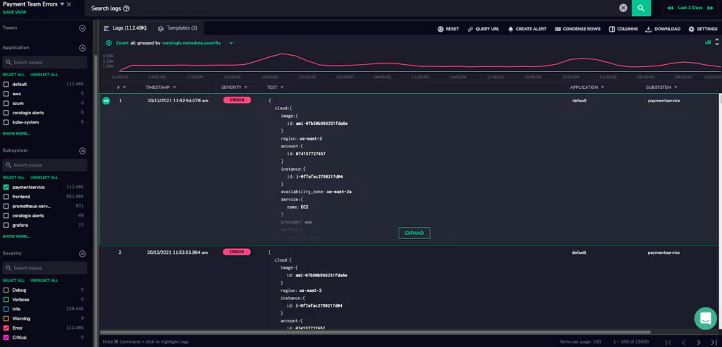
For example, the first Logs View that we defined filtered for Error and Critical level logs from our team’s applications and subsystems.
One of the existing errors that we tackled immediately was timeouts of internal HTTP requests between our services. For handling these kinds of errors, we improved the efficiency of SQL queries and in-memory calculations and adopted better configuration for our HTTP clients and servers.
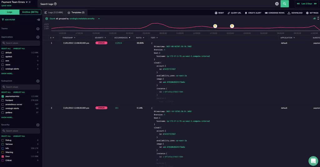
2. Use templates to consolidate logs into a single issue.
Using the Logs Screen to investigate issues, we rely on Coralogix’s Loggregation feature which deduplicates our noisy logs into more manageable templates. This way we can look at issues as a whole rather than individual log lines.
When we created our Log View, we were looking at more than 100K log errors, but many of those were from the same issue. Looking at the log templates, it was easy to see that only 2 issues were causing all of those errors, and we were able to immediately fix them and clear the service.
Zero-Error Policy with Coralogix
1. Define a Coralogix Alert from your view.
To really implement a zero-error policy, it’s important to stay on top of new errors as they come up. To do this with Coralogix, we created an alert directly from our Log View to be fired for the same filters with a summary of errors grouped by subsystem. We also defined an alert to be triggered immediately after each error.
Using our Webhook integration with Slack, we easily centralized these alert notifications in a dedicated Slack channel and added all relevant team members. Using Jira integration for Slack, we can also create Jira tickets for each encountered issue.
Known and non-urgent issues are filtered out from the alert, changed into Info/Warning severity, or deleted.
Now, after each fix and deployment, we are immediately aware of its impact. When the error has been resolved, the alert will not be triggered anymore. If we add a fix that doesn’t work, we get additional alerts triggering for the same issue or may see another new issue that may have been accidentally added while fixing the first one.
Summary
After applying the steps above and ensuring our system is clear from errors, we have reached a state where we can immediately identify every new error and reduce the total number of alerts and bugs which affect our customers. After the first cleanup, our team’s number of high urgency incidents was reduced by 30%. That helped us to stay focused on our day-to-day work, with fewer interruptions resulting from urgent issues.
We’ve moved the notifications of the Coralogix alerts we created to our team channel, along with other defined Coralogix and Prometheus alerts. This was done in order to keep the engagement of the entire team on new errors and alerts and to facilitate maintaining the zero-error policy. Today, all alerts are being identified, assigned, and fixed by our team in a transparent and efficient way.
Logging solutions are a must-have for any company with software systems. They are necessary to monitor your software solution’s health, prevent issues before they happen, and troubleshoot existing problems.
The market has many solutions which all focus on different aspects of the log monitoring problem. These solutions include both open source and proprietary software and tools built into cloud provider platforms, and give a variety of different features to meet your specific needs. Grafana Loki is a relatively new industry solution so let’s take a closer look at what it is, where it came from, and if it might meet your logging needs.
What is Grafana Loki, and Where Did it Come From?
Grafana Loki based its architecture on Prometheus’s use of labels to index data. Doing this allows Loki to store indexes in less space. Further, Loki’s design directly plugs into Prometheus, meaning developers can use the same label criteria with both tools.
Prometheus is open source and has become the defacto standard for time-series metrics monitoring solutions. Being a cloud-native solution, developers primarily use Prometheus when software is built with Kubernetes or other cloud-native solutions.
Prometheus is unique in its capabilities of collecting multi-dimensional data from multiple sources, making it an attractive solution for companies running microservices on the cloud. It has an alerting system for metrics, but developers often augment it with other logging solutions. Other logging solutions tend to give more observability into software systems and add a visualization component to the logs.
Prometheus created a new query language (PromQL), making it challenging to visualize logging for troubleshooting and monitoring. Many of the available logging solutions were built before Prometheus came to the logging scene in 2012 and did not support linking to Prometheus.
What Need does Grafana Loki Fill?
Grafana Loki was born out of a desire to have an open source tool that could quickly select and search time-series logs where the logs are stored stably. Discerning system issues may include log visualization tools with a querying ability, log aggregation, and distributed log tracing.
Existing open source tools do not easily plug into Prometheus for troubleshooting. They did not allow developers to search for Prometheus’s metadata for a specific period, instead only allowing them to search the most recent logs this way. Further, log storage was not efficient, so developers could quickly max out their logging limits and need to consider which logs they could potentially live without. With some tools, crashes could mean that logs are lost forever.
It’s important to note that there are proprietary tools on the market that do not have these same limitations and have capabilities far beyond what open source tools are capable of providing. These tools can allow for time-bound searching, log aggregation, and distributed tracing with a single tool instead of using a separate open source tool for each need. Coralogix, for example, allows querying of logs using SQL queries or Kibana visualizations and also ingests Prometheus metrics along with metrics from several other sources.
Grafana Loki’s Architecture
Built from Components
Developers built Loki’s service from a set of components (or modules). There are four components available for use: distributor, ingester, querier, and query frontend.
Distributor
The distributor module handles and validates incoming data streams from clients. Valid data is chunked and sent to multiple ingesters for parallel processing.
The distributor relies on Prometheus-like labels to validate log data in the distributor and to process in different downstream modules. Without labels, Grafana Loki cannot create the index it requires for searching. Suppose your logs do not have appropriate labels, for example. In that case, if you are loading from services other than Prometheus, the Loki architecture may not be the optimal choice for log aggregations.
Ingester
The ingester module writes data to long-term storage. Loki does not store the log data it ingests, instead only indexing metadata. The object storage used is configurable, for example, AWS S3, Apache Cassandra, or local file systems.
The ingester also returns data for in-memory queries. Ingester crashes cause unflushed data to be lost. Loki can irretrievably lose logs from ingesters with improper user setup ensuring redundancy.
Querier
Grafana Loki uses the querier module to handle the user’s queries on the ingester and the object stores. Queries are run first against local storage and then against long-term storage. The querier must handle duplicate data because it queries multiple places, and the ingesters do not detect duplicate logs in the writing process. The querier has an internal mechanism, so it returns data with the same timestamp, label data, and log data only once.
Query Frontend
The query frontend module optionally gives API endpoints for queries that enable parallelization of large queries. The query frontend still uses queries, but it will split a large query into smaller ones and execute the reads on logs in parallel. This ability is helpful if you are testing out Grafana Loki and do not yet want to set up a querier in detail.
Object Stores
Loki needs long-term data storage for holding queryable logs. Grafana Loki requires an object store to hold both compressed chunks written by the ingester and the key-value pairs for the chunk data. Fetching data from long-term storage can take more time than local searches.
The file system is the only no-added-cost option available for storing your chunked logs, with all others belonging to managed object stores. The file system comes with downsides since it is not scalable, not durable, and not highly available. It’s recommended to use the file system storage for testing or development only, not for troubleshooting in production environments.
There are many other log storage options available that are scalable, durable, and highly available. These storage solutions accrue costs for reading and writing data and data storage. Coralogix, a proprietary observability platform, analyzes data immediately after ingestion (before indexing and storage) and then charges based on how the data will be used. This kind of pricing model reduces hidden or unforeseen costs that are often associated with Cloud storage models.
Grafana Loki’s Feature Set
Horizontally Scalable
Developers can run Loki in one of two modes depending on the target value. When developers set the target to all, Loki runs components on a single server in monolith mode. Setting the target to one of the available component names runs Loki in a horizontally-scalable or microservices mode where a server is available for each component.
Users can scale distributors, ingestors, and querier components as needed to handle the size of their stored logs and the speed of responses.
Inexpensive Log Storage and Querying
Being open source, Grafana Loki is an inexpensive option for log analytics. The cost involved with using the free-tier cloud solution, or the source code installed through Tanka or Docker, is in storing the log and label data.
Loki recommends labels be kept as small as possible to keep querying fast. As a result, label stores can be relatively small compared to the complete log data. Complete logs are compressed with your choice of the tool before being stored, making the storage even more efficient.
Note: Compression tools generally have a tradeoff between storage size and read speed, meaning developers will need to consider cost versus speed when setting up their Loki system.
Grafana uses Cloud storage solutions like AWS S3 or Google’s GCS. Loki’s cost depends on the size of logs needed for analysis and the frequency of read/write operations. For example, AWS S3 charges for each GB stored and for each request made against the S3 bucket.
Fast Querying
When logs are imported into Grafana Loki using Promtail, ingesters split out labels from the log data. Labels should be as limited as possible since they are used to select logs searched during queries. An implicit requirement of getting speedy queries with Loki is concise and limited labels.
When you query, Loki splits data according to time and then sharded by the index. Available queriers are then applied to read the shard’s entire contents looking for the given search parameters. The more queriers available and the smaller the index, the faster the query response will be available.
Grafana Loki uses brute force along with parallelized components to gain speed of querying. This speed gained with Grafana Loki is considerable for a brute force methodology. Loki uses this brute-force method to gain simplicity over fully indexed solutions. However, fully indexed solutions can search logs more robustly.
Open Source
Open source solutions like Grafana Loki always have drawbacks. The Loki team has had a great interest in their product and works diligently to address the new platform’s issues. Grafana Loki relies on community assistance with documentation and features. Community reliance means setting up and enhancing a log analytics platform with Loki can take significant and unexpected developer resources.
To ensure speedy responses, users must sign up for Enterprise services which come at a cost like other proprietary systems. If you are considering these Enterprise services, ensure you have looked at other proprietary solutions, so you get the most valuable features from your log analytics platform.
Summary
Grafana Loki is an open source, horizontally scalable, brute-force log aggregation tool built for use with Prometheus. Production users will need to combine Loki with a cloud account for log storage.
Loki gives users a low barrier-to-entry tool that plugs into both Prometheus for metrics and Grafana for log visualization in a simple way. The free version does have drawbacks since it is not guaranteed to be available. There are also instances where Loki can lose logs without proper redundancy implemented.
Proprietary tools are also available with Grafana Loki’s features and with added log aggregation and analytics features. One such tool is the Coralogix observability platform which offers real-time analytics, anomaly detection, and a developer-friendly live tail with CLI.
For the seasoned user, PromQL confers the ability to analyze metrics and achieve high levels of observability. Unfortunately, PromQL has a reputation among novices for being a tough nut to crack.
Fear not! This PromQL tutorial will show you five paths to Prometheus godhood. Using these tricks will allow you to use Prometheus with the throttle wide open.
Aggregation
Aggregation is a great way to construct powerful PromQL queries. If you’re familiar with SQL, you’ll remember that GROUP BY allows you to group results by a field (e.g country or city) and apply an aggregate function, such as AVG() or COUNT(), to values of another field.
Aggregation in PromQL is a similar concept. Metric results are aggregated over a metric label and processed by an aggregation operator like sum().
Aggregation Operators
PromQL has twelve built in aggregation operators that allow you to perform statistics and data manipulation.
Group
What if you want to aggregate by a label just to get values for that label? Prometheus 2.0 introduced the group() operator for exactly this purpose. Using it makes queries easier to interpret and means you don’t need to use bodges.
Count those metrics
PromQL has two operators for counting up elements in a time series. Count() simply gives the total number of elements. Count_values() gives the number of elements within a time series that have a specified value. For example, we could count the number of binaries running each build version with the query:
count_values("version", build_version)
Sum() does what it says. It takes the elements of a time series and simply adds them all together. For example if we wanted to know the total http requests across all our applications we can use:
sum(http_requests_total)
Stats
PromQL has 8 operators that pack a punch when it comes to stats.
Avg() computes the arithmetic mean of values in a time series.
Min() and max() calculate the minimum and maximum values of a time series. If you want to know the k highest or lowest values of a time series, PromQL provides topk() and bottomk(). For example if we wanted the 5 largest HTTP requests counts across all instances we could write:
topk(5, http_requests_total)
Quantile() calculates an arbitrary upper or lower portion of a time series. It uses the idea that a dataset can be split into ‘quantiles’ such as quartiles or percentiles. For example, quantile(0.25, s) computes the upper quartile of the time series s.
Two powerful operators are stddev(), which computes the standard deviation of a time series and stdvar, which computes its variance. These operators come in handy when you’ve got application metrics that fluctuate, such as traffic or disk usage.
By and Without
The by and without clauses enable you to choose which dimensions (metric labels) to aggregate along. by tells the query to include labels: the query sum by(instance)(node_filesystem_size_bytes) returns the total node_filesystem_size_bytes for each instance.
In contrast, withouttells the query which labels not to include in the aggregation. The query sum without(job) (node_filesystem_size_bytes) returns the total node_filesystem_size_bytes for all labels except job.
Joining Metrics
SQL fans will be familiar with joining tables to increase the breadth and power of queries. Likewise, PromQL lets you join metrics. As a case in point, the multiplication operator can be applied element-wise to two instance vectors to produce a third vector.
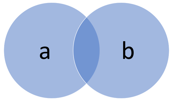
Let’s look at this query which joins instance vectors a and b.
a * b
This makes a resultant vector with elements a1b1, a2b2… anbn . It’s important to realise that if a contains more elements than b or vice versa, the unmatched elements won’t be factored into the resultant vector.
This is similar to how an SQL inner join works; the resulting vector only contains values in both a and b.
Joining Metrics on Labels
We can change the way vectors a and b are matched using labels. For instance, the querya * on (foo, bar) group_left(baz) b matches vectors a and b on metric labels foo and bar. (group_left(baz) means the result contains baz, a label belonging to b.
Conversely you can use ignoring to specify which label you don’t want to join on. For example the query a * ignoring (baz) group_left(baz) bjoins a and b on every label except baz. Let’s assume a contains labels foo and bar and b contains foo, bar and baz. The query will join a to b on foo and bar and therefore be equivalent to the first query.
Later, we’ll see how joining can be used in Kubernetes.
Labels: Killing Two Birds with One Metric
Metric labels allow you to do more with less. They enable you to glean more system insights with fewer metrics.
Scenario: Using Metric Labels to Count Errors
Let’s say you want to track how many exceptions are thrown in your application. There’s a noob way to solve this and a Prometheus god way.
The Noob Solution
One solution is to create a counter metric for each given area of code. Each exception thrown would increment the metric by one.
This is all well and good, but how do we deal with one of our devs adding a new piece of code? In this solution we’d have to add a corresponding exception-tracking metric. Imagine that barrel-loads of code monkeys keep adding code. And more code. And more code.
Our endpoint is going to pick up metric names like a ship picks up barnacles. To retrieve the total exception count from this patchwork quilt of code areas, we’ll need to write complicated PromQL queries to stitch the metrics together.
The God Solution
There’s another way. Track the total exception count with a single application-wide metric and add metric labels to represent new areas of code. To illustrate, if the exception counter was called “application_error_count” and it covered code area “x”, we can tack on a corresponding metric label.
application_error_count{area="x"}
As you can see, the label is in braces. If we wanted to extend application_error_count’s domain to code area “y”, we can use the following syntax.
application_error_count{area="x|y"}
This implementation allows us to bolt on as much code as we like without changing the PromQL query we use to get total exception count. All we need to do is add area labels.
If we do want the exception count for individual code areas, we can always slice application_error_count with an aggregate query such as:
count by(application_error_count)(area)
Using metric labels allows us to write flexible and scalable PromQL queries with a manageable number of metrics.
Manipulating Labels
PromQL’s two label manipulation commands are label_join and label_replace.label_join allows you to take values from separate labels and group them into one new label. The best way to understand this concept is with an example.
In this query, the values of three labels, src1, src2 and src3 are grouped into label foo. Foo now contains the respective values of src1, src2 and src3 which are a, b, and c.
label_replacerenames a given label. Let’s examine the query
This query replaces the label “service” with the label “foo”. Now foo adopts service’s value and becomes a stand in for it. One use of label_replace is writing cool queries for Kubernetes.
Creating Alerts with predict_linear
Introduced in 2015, predict_linear is PromQL’s metric forecasting tool. This function takes two arguments. The first is a gauge metric you want to predict. You need to provide this as a range vector. The second is the length of time you want to look ahead in seconds.
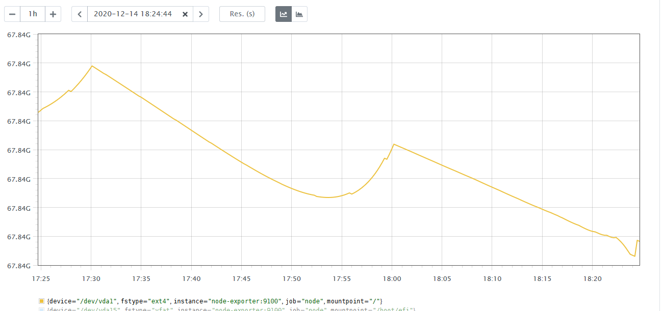
predict_linear takes the metric at hand and uses linear regression to extrapolate forward to its likely value in the future. As an example, let’s use PromLens to run the query:
It shows a graph which shows the predicted value an hour from the current time.
Alerts and predict_linear
The main use of predict_linear is in creating alerts. Let’s imagine you want to know when you run out of disk space. One way to do this would be an alert which fires as soon as a given disk usage threshold is crossed. For example, you might get alerted as soon as the disk is 80% full.
Unfortunately, threshold alerts can’t cope with extremes of memory usage growth. If disk usage grows slowly, it makes for noisy alerts. An alert telling you to urgently act on a disk that’s 80% full is a nuisance if disk space will only run out in a month’s time.
If, on the other hand, disk usage fluctuates rapidly, the same alert might be a woefully inadequate warning. The fundamental problem is that threshold-based alerting knows only the system’s history, not its future.
In contrast, an alert based on predict_linear can tell you exactly how long you’ve got before disk space runs out. Plus, it’ll even handle left curves such as sharp spikes in disk usage.
Scenario: predict_linear in action
This wouldn’t be a good PromQL tutorial without a working example, so let’s see how to implement an alert which gives you 4 hours notice when your disk is about to fill up. You can begin creating the alert using the following code in a file “node.rules”.
This is a PromQL expression using predict_linear. node_filesystem_free is a gauge metric measuring the amount of memory unused by your application. The expression is performing linear regression over the last hour of filesystem history and predicting the probable free space. If this is less than zero the alert is triggered.
The line after this is a failsafe, telling the system to test predict_linear twice over a 5 minute interval in case a spike or race condition gives a false positive.
Using PromQL’s predict_linear function leads to smarter, less noisy alerts that don’t give false alarms and do give you plenty of time to act.
Putting it All Together: Monitoring CPU Usage in Kubernetes
To finish off this PromQL tutorial, let’s see how PromQL can be used to create graphs of CPU-utilisation in a Kubernetes application.
In Kubernetes, applications are packaged into containers and containers live on pods. Pods specify how many resources a container can use. If a container uses more resources than its pod has, it ‘spills over’ into a second pod.
This means that a candidate PromQL query needs the ability to sum over multiple pods to get the total resources for a given container. Our query should come out with something like the following.
Container
CPU utilisation per second
redash-redis
0.5
redash-server-gunicorn
0.1
Aggregating by Pod Name
We can start by creating a metric of CPU usage for the whole system, called container_cpu_usage_seconds_total. To get the CPU utilisation per second for a specific namespace within the system we use the following query which uses PromQL’s rate function:
This is where aggregation comes in. We can wrap the above query in a sum query that aggregates over the pod name.
sum by(pod_name)( rate(container_cpu_usage_seconds_total{namespace= “redash”[5m]))
So far, our query is summing the CPU usage rate for each pod by name.
Retrieving Pod Labels
For the next step, we need to get the pod labels, “pod” and “label_app”. We can do this with the query:
group(kube_pod_labels{label_app=~”redash-*”}) by (label_app, pod)
By itself, kube_pod_labels returns all existing labels. The code between the braces is a filter acting on label_app for values beginning with “redash-”.
We don’t, however, want all the labels, just label_app and pod. Luckily, we can exploit the fact that pod labels have a value of 1. This allows us to use group() to aggregate along the two pod labels that we want. All the others are dropped from the results.
Joining Things Up
So far, we’ve got two aggregation queries. Query 1 uses sum() to get CPU usage for each pod. Query 2 filters for the label names label_app and pod. In order to get our final graph, we have to join them up. To do that we’re going to use two tricks, label_replace() and metric joining.
The reason we need label replace is that at the moment query 1 and query 2 don’t have any labels in common. We’ll rectify this by replacing pod_name with pod in query 1. This will allow us to join both queries on the label “pod”. We’ll then use the multiplication operator to join the two queries into a single vector.
We’ll pass this vector into sum() aggregating along label app. Here’s the final query:
Hopefully this PromQL tutorial has given you a sense for what the language can do. Prometheus takes its name from a Titan in Greek mythology, who stole fire from the gods and gave it to mortal man. In the same spirit, I’ve written this tutorial to put some of the power of Prometheus in your hands.
You can put the ideas you’ve just read about into practice using the resources below, which include online code editors to play with the fire of PromQL at your own pace.
This online editor allows you to get started with PromQL without downloading Prometheus. As well as tabular and graph views, there is also an “explain” view. This gives the straight dope on what each function in your query is doing, helping you understand the language in the process.
This tutorial by Coralogix explains how to integrate your Grafana instance with Coralogix, or you can use our hosted Grafana instance that comes automatically connected to your Coralogix data.
This tutorial will demonstrate how to integrate your Prometheus instance with Coralogix, to take full advantage of both a powerful open source solution and one of the most cutting edge SaaS products on the market.
Prometheus metrics are an essential part of your observability stack. Observability comes hand in hand with monitoring, and is covered extensively here in this Essential Observability Techniques article.A well-monitored application with flexible logging frameworks can pay enormous dividends over a long period of sustained growth, but Prometheus has a problem when it comes to scale.
Prometheus Metrics at Scale
Prometheus is an extremely popular choice for collecting and querying real-time metrics primarily due to its simplicity, ease of integration, and powerful visualizations. It’s perfect for small and medium-sized applications, but what about when it comes to scaling?
Unfortunately, a traditional Prometheus & Kubernetes combo can struggle at scale given its heavy reliance on writing memory to disk. Without specialized knowledge in the matter, configurations for high performance at scale is extremely tough. For example, querying through petabytes of historical data with any degree of speed will prove to be extremely challenging with a traditional Prometheus setup as it relies heavily on read/write disk operations.
So how do you scale your Prometheus Metrics?
This is where Thanos comes to the rescue. In this article, we will be expanding upon what Thanos is, and how it can give us a helping hand and allow us to scale using Prometheus without the memory headache. Lastly, we will be running through a few great usages of Thanos and how effective it is using real world examples as references.
Thanos
Thanos, simply put, is a “highly available Prometheus setup with long-term storage capabilities”. The word “Thanos” comes from the Greek “Athanasios”, meaning immortal in English. True to its name, Thanos features object storage for an unlimited time and is heavily compatible with Prometheus and other tools that support it such as grafana.
Thanos allows you to aggregate data from multiple Prometheus instances and query them, all from a single endpoint. Thanos also automatically deals with duplicate metrics that may arise from multiple Prometheus instances.
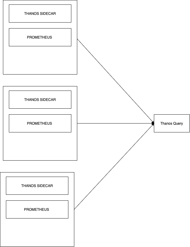
Let’s say we were running multiple prometheus instances, and wanted to use Thanos to our advantage. We will take a look at the relationship between these two components and then delve into more technical details.
Storage
The first step to solving memory woes using Thanos is its Sidecar component, as it allows seamless uploading of metrics as object storage on your typical providers (S3, Swift, Azure etc). It employs the use of the StoreAPI as an API gateway, and only uses a small amount of disk space to keep track of remote blocks and keep them in sync. The StoreAPI is a gRPC that uses SSL/TLS authentication, and therefore standard HTTP operations are converted into gRPC format. Information on this can be found here.
Thanos also features Time Based Partitioning which allows you to set flags that query metrics from certain timeframes within the Store Gateway. For example: --min-time=-6w would be used as a flag to filter data older than 6 weeks.
Additionally, Thanos has an Index Cache and implements the use of a Caching Bucket – certainly powerful features that allow you to safely transition from a read/write dependency to seamless cloud storage. These latency performance boosters are essential when scaling – every ms counts.
The use of the Sidecar is also invaluable in case of an outage. It is key to be able to refer to historical data through the use of backups on the cloud. Using a typical Prometheus setup, you could very well lose important data in case of an outage.
Basic Thanos Query
The basic Thanos setup seen above in the diagram also contains the Thanos Query component, which is responsible for aggregating and deduplicating metrics like briefly mentioned earlier. Similar to storage, Thanos Query also employs the use of an API – namely the Prometheus HTTP API. This allows querying data within a Thanos cluster via PromQL. It intertwines with the previously mentioned StoreAPI by querying underlying objects and returning the result. The Thanos querier is “fully stateless and horizontally scalable”, per its developers.
Scaling Thanos Query
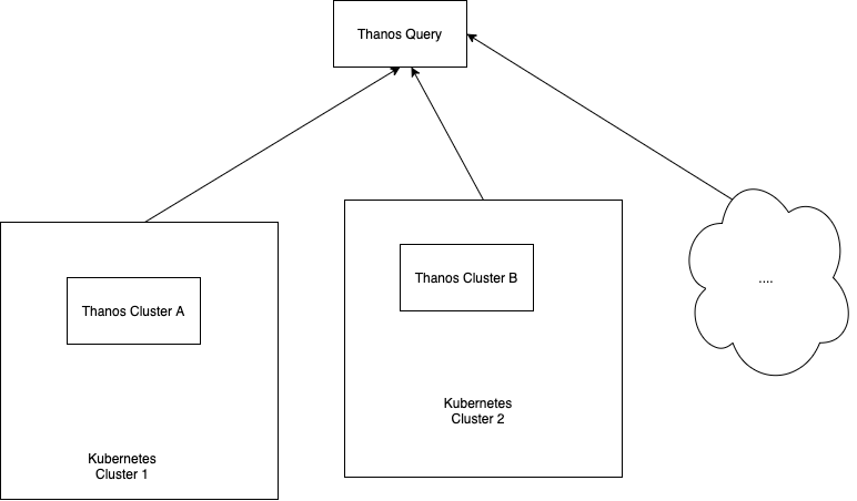
Thanos Query works as an aggregator for multiple sidecar instances, but we could easily find ourselves using multiple Kubernetes clusters, with multiple Prometheus instances. This would mean we would have multiple Thanos Query nodes leading subsets of Sidecar & Prometheus instances. Intuitively, this is a difficult problem to solve.
The good news is that a Thanos Query node aggregates multiple instances of Thanos Query nodes also! Sounds confusing? It’s actually very simple:
It doesn’t matter if your project spans over multiple Kubernetes clusters. Thanos deduplicates metrics automatically. The “head” Thanos Query node takes care of this for us by running high performance deduplication algorithms.
The clear advantage to this type of setup is that we end up with a single node where we can query all of our metrics. But this also has a clear disadvantage – What if our head Thanos Query node goes down? Bye bye metrics?
Luckily there are options to truly nail the Thanos setup over multiple Kubernetes clusters. This fantastic article runs through “Yggdrasil”, an AWS multi-cluster load-balancing tool. It allows you to perform queries against any of your clusters and still access all of your metrics. This is especially important in case of any downtime or service failures. With careful planning, you can cut down data loss to pretty much near 0%.
Availability
It should be clear by now that the sum of all these parts is a Prometheus setup with high availability of data. The use of Thanos Query and Thanos Sidecar significantly facilitate the availability of objects and metrics. Given the convenience of a single metric collection point, alongside unlimited retention of object storage, it’s easy to see why the first four words on the Thanos website are “Highly available Prometheus setup”.
Uses of Thanos for Prometheus Metrics
Nubank
Many large companies are using Thanos to their advantage. Nubank, a Brazilian fintech company that toppled a $10B valuation last year, has seen massive increases to operational efficiency after fitting Thanos, within other tools into their tech stack.
A case study on the company revealed that the Nubank cloud native platform “includes Prometheus, Thanos and Grafana for monitoring”. Although its ultimately impossible to attribute this solely to Thanos, the case study explains how Nubank now deploys “700 times a week” and has “gained about a 30% cost efficiency”. It seems even a very large-scale application can deeply benefit from a hybrid Prometheus+Thanos setup.
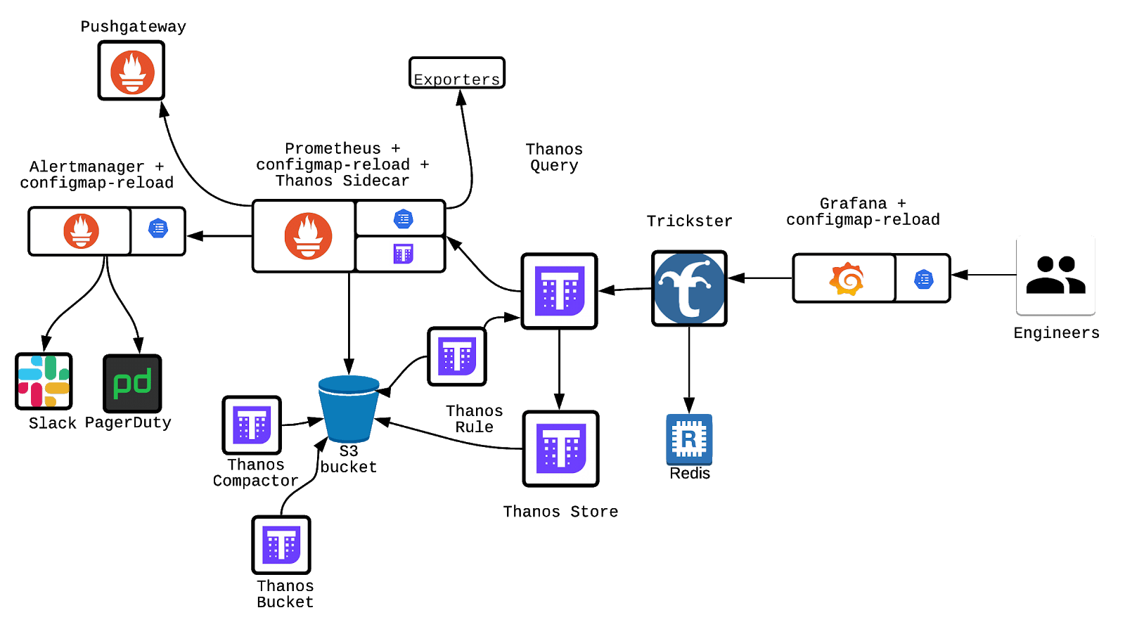
GiffGaff
Popular UK mobile network provider GiffGaff also boasts the use of Thanos. In fact, they have been fairly public as to how Thanos fits into their stack and what sort of advantages it has given them.
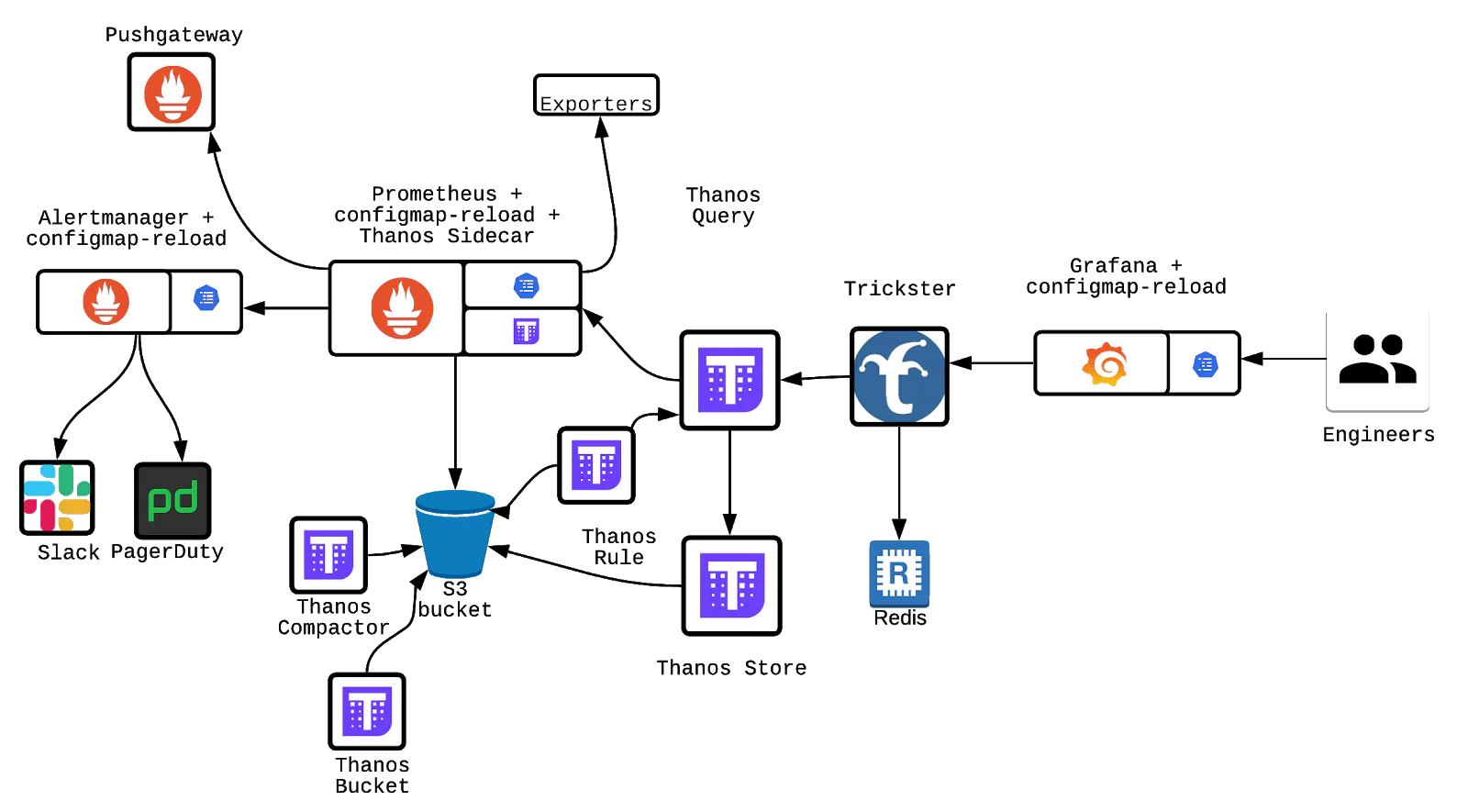
The diagram above shows that the Thanos Store, Thanos Query and Thanos Bucket. They are critical parts of the monitoring data flow. Objects are constantly being synced and uploaded onto an S3 bucket. In comparison to disk operations seen in a normal Prometheus setup, this scales far more and benefits from the reliability of S3.
Within their post under the “Thanos” section, GiffGaff claims “As long as at least one server is running at a given time, there shouldn’t be data loss.” This hints at some form of multi-cluster load balancing at the very least.
“… [Thanos] allowed us [GiffGaff] to retain data for very long periods in a cost-efficient way”
Interestingly, GiffGaff employs the use of the sidecar to upload objects every 2 hours – hedging against any potential prometheus downtime.
GiffGaff uses Thanos Store and allocates time periods for each Thanos Store cluster for storage. This effectively rotates the cluster use, keeping availability and reliability very high. The example given, by GiffGaff themselves is:
now – 2h: Thanos Sidecars
2h – 1 month: Thanos Store 1
1 month – 2 months: Thanos Store 2
2 months – 3 months: Thanos Store 3
We had previously touched upon Thanos downsampling and how it could save you time when querying historical data. In order to implement this, GiffGaff used the Thanos Compactor, “performing 5m downsampling after 40 hours and 1h downsampling after 10 days.” Impressive to say the least.
Conclusion
Now you know what Thanos is, how it interacts with Prometheus and the type of advantages it can give us. In this post, we also ran through some real life examples which should give some insight into how Thanos is used. It should also be clear how the use of Thanos Sidecar and Storage are inherently advantageous when it comes to scaling, in relation to a typical Prometheus setup.
Apart from storage capabilities, the effectiveness of Thanos Query should also be direct – and how a single metric collection point is a massive blessing but comes with its own responsibilities should you need to balance the load on multiple clusters.
Lastly, downsampling through the use of the Thanos Compactor seems like a performance no brainer. Large datasets can be easily handled using the downsampling method.
Hopefully you understand Thanos and what it has to offer to make your life easier. If that sounds like a lot of work, Coralogix offers a powerful suite of monitoring tools.
Kubernetes log monitoring can be complex. To do it successfully requires several components to be monitored simultaneously. First, it’s important to understand what those components are, which metrics should be monitored and what tools are available to do so.
In this post, we’ll take a close look at everything you need to know to get started with monitoring your Kubernetes-based system.
Monitoring Kubernetes Clusters vs. Kubernetes Pods
Monitoring Kubernetes Clusters
When monitoring the cluster, a full view across all areas is obtained, giving a good impression of the health of all pods, nodes, and apps.
Key areas to monitor at the cluster level include:
Node load: Tracking the load on each node is integral to monitoring efficiency. Some nodes are used more than others. Rebalancing the load distribution is key to keeping workloads fluid and effective. This can be done via DaemonSets.
Unsuccessful pods: Pods fail and abort. This is a normal part of Kubernetes processes. When a pod that should be working at a more efficient level or is inactive, it is essential to investigate the reason behind the anomalies in pod failures.
Cluster usage: Monitoring cluster infrastructure allows adjustment of the number of nodes in use and the allocation of resources to power workloads efficiently. The visibility of resources being distributed allows scaling up or down and avoids the costs of additional infrastructure. It is important to set a container’s memory and CPU usage limit accordingly.
Monitoring Kubernetes Pods
Cluster monitoring provides a global view of the Kubernetes environment, but collecting data from individual pods is also essential. It reveals the health of individual pods and the workloads they are hosting, providing a clearer picture of pod performance at a granular level, beyond the cluster.
Key areas to monitor at the cluster level include:
Total pod instances: There needs to be enough instances of a pod to ensure high availability. This way hosting bandwidth is not wasted, however consideration is needed to not run ‘too many extra’ pod instances.
Actual pod instances: Monitoring the number of instances for each pod that’s running versus what is expected to be running will reveal how to redistribute resources to achieve the desired state in terms of pods instances. ReplicaSets could be misconfigured with varying metrics, so it’s important to analyze these regularly.
Pod deployment: Monitoring pods deployment allows to view any misconfigurations that might be diminishing the availability of pods. It’s critical to monitor how resources distribute to nodes.
Important Metrics for Kubernetes Monitoring
To gain a higher visibility into a Kubernetes installation, there are several metrics that will provide valuable insight into how the apps are running.
Common metrics
These are metrics collected from the Kubernetes code, written in Golang. They allow understanding of performance in the platform at a cellular level and display the state of what is happening in the GoLang processes.
Node metrics –
Monitoring the standard metrics from the operating systems that power Kubernetes nodes provides insight into the health of each node.
Each Kubernetes Node has a finite capacity of memory and CPU and that can be utilized by the running pods, so these two metrics need to be monitored carefully. Other common node metrics to monitor include CPU load, memory consumption, filesystem activity and usage and network activity.
One approach to monitoring all cluster nodes is to create a special kind of Kubernetes pod called DaemonSets. Kubernetes ensures that every node created has a copy of the DaemonSet pod, which virtually enables one deployment to watch each machine in the cluster. As nodes are destroyed, the pod is also terminated.
Kubelet metrics –
To ensure the Control Plane is communicating efficiently with each individual node that a Kubelet runs on, it is recommended to monitor the Kubelet agent regularly. Beyond the common GoLang common metrics described above, Kubelet exposes some internals about its actions that are useful to track as well.
Controller manager metrics –
To ensure that workloads are orchestrated effectively, monitor the requests that the Controller is making to external APIs. This is critical in cloud-based Kubernetes deployments.
Scheduler metrics
To identify and prevent delays, monitor latency in the scheduler. This will ensure Kubernetes is deploying pods smoothly and on time.
The main responsibility of the scheduler is to choose which nodes to start newly launched pods on, based on resource requests and other conditions.
The scheduler logs are not very helpful on their own. Most of the scheduling decisions are available as Kubernetes events, which can be logged easily in a vendor-independent way, thus are the recommended source for troubleshooting. The scheduler logs might be needed in the rare case when the scheduler is not functioning, but a kubectl logs call is usually sufficient.
etcd metrics –
etcd stores all the configuration data for Kubernetes. etcd metrics will provide essential visibility into the condition of the cluster.
Container metrics –
Looking specifically into individual containers will allow monitoring of exact resource consumption rather than more general Kubernetes metrics. CAdvisor analyzes resource usage happening inside containers.
API Server metrics –
The Kubernetes API server is the interface to all the capabilities that Kubernetes provides. The API server controls all the operations that Kubernetes can perform. Monitoring this critical component is vital to ensure a smooth running cluster.
The API server metrics are grouped into a major categories:
Request Rates and Latencies
Performance of controller work queues
etcd helper cache work queues and cache performance
General process status (File Descriptors/Memory/CPU Seconds)
Golang status (GC/Memory/Threads)
kube-state-metrics –
kube-state-metrics is a service that makes cluster state information easily consumable. Where the Metrics Server exposes metrics on resource usage by pods and nodes, kube-state-metrics listens to the Control Plane API server for data on the overall status of Kubernetes objects (nodes, pods, Deployments, etc) as well as the resource limits and allocations for those objects. It then generates metrics from that data that are available through the Metrics API.
kube-state-metrics is an optional add-on. It is very easy to use and exports the metrics through an HTTP endpoint in a plain text format. They were designed to be easily consumed / scraped by open source tools like Prometheus.
In Kubernetes, the user can fetch system-level metrics from various out of the box tools like cAdvisor, Metrics Server, and Kubernetes API Server. It is also possible to fetch application level metrics from integrations like kube-state-metrics and Prometheus Node Exporter.
Prometheus scrapes metrics from instrumented jobs, either directly or via an intermediary push gateway for short-lived jobs. It locally stores all scraped samples and runs rules over this data to either aggregate and record new time series from existing data or generate alerts. Grafana or other API tools can be used to visualize the collected data.
Prometheus, Grafana and Alertmanager
One of the most popular Kubernetes monitoring solutions is the open-source Prometheus, Grafana and Alertmanager stack, deployed alongside kube-state-metrics and node_exporter to expose cluster-level Kubernetes object metrics as well as machine-level metrics like CPU and memory usage.
What is Prometheus?
Prometheus is a pull-based tool used specifically for containerized environments like Kubernetes. It is primarily focused on the metrics space and is more suited for operational monitoring. Exposing and scraping prometheus metrics is straightforward, and they are human readable, in a self-explanatory format. The metrics are published using a standard HTTP transport and can be checked using a web browser.
Apart from application metrics, Prometheus can collect metrics related to:
Node exporter, for the classical host-related metrics: cpu, mem, network, etc.
Kube-state-metrics for orchestration and cluster level metrics: deployments, pod metrics, resource reservation, etc.
Kube-system metrics from internal components: kubelet, etcd, scheduler, etc.
Prometheus can configure rules to trigger alerts using PromQL, Alertmanager will be in charge of managing alert notification, grouping, inhibition, etc.
Using Prometheus with Alertmanager and Grafana
PromQL (Prometheus Query Language) lets the user choose time-series data to aggregate and then view the results as tabular data or graphs in the Prometheus expression browser. Results can also be consumed by the external system via an API.
How does Alertmanager fit in? The Alertmanager component configures the receivers, gateways to deliver alert notifications. It handles alerts sent by client applications such as the Prometheus server and takes care of deduplicating, grouping, and routing them to the correct receiver integration such as email, PagerDuty or OpsGenie. It also takes care of silencing and inhibition of alerts.
Grafana can pull metrics from any number of Prometheus servers and display panels and dashboards. It also has the added ability to register multiple different backends as a datasource and render them all out on the same dashboard. This makes Grafana an outstanding choice for monitoring dashboards.
Useful Log Data for Troubleshooting
Logs are useful to examine when a problem is revealed by metrics. They give exact and invaluable information which provides more details than metrics. There are many options for logging in most of Kubernetes’ components. Applications also generate log data.
Digging deeper into the cluster requires logging into the relevant machines.
The locations of the relevant log files are:
Master
/var/log/kube-apiserver.log – API Server, responsible for serving the API
/var/log/kube-scheduler.log – Scheduler, responsible for making scheduling decisions
/var/log/kube-controller-manager.log – Controller that manages replication controllers
Worker nodes
/var/log/kubelet.log – Kubelet, responsible for running containers on the node
/var/log/kube-proxy.log – Kube Proxy, responsible for service load balancing
etcd logs
etcd uses the Github capnslog library for logging application output categorized into levels.
A log message’s level is determined according to these conventions:
Error: Data has been lost, a request has failed for a bad reason, or a required resource has been lost.
Warning: Temporary conditions that may cause errors, but may work fine.
Notice: Normal, but important (uncommon) log information.
Info: Normal, working log information, everything is fine, but helpful notices for auditing or common operations.
Debug: Everything is still fine, but even common operations may be logged and less helpful but more quantity of notices.
kubectl
When it comes to troubleshooting the Kubernetes cluster and the applications running on it, understanding and using logs are crucial. Like most systems, Kubernetes maintains thorough logs of activities happening in the cluster and applications, which highlight the root causes of any failures.
Logs in Kubernetes can give an insight into resources such as nodes, pods, containers, deployments and replica sets. This insight allows the observation of the interactions between those resources and see the effects that one action has on another. Generally, logs in the Kubernetes ecosystem can be divided into the cluster level (logs outputted by components such as the kubelet, the API server, the scheduler) and the application level (logs generated by pods and containers).
Use the following syntax to run kubectl commands from your terminal window:
kubectl [command] [TYPE] [NAME] [flags]
Where:
command: the operation to perform on one or more resources, i.e. create, get, describe, delete.
TYPE: the resource type.
NAME: the name of the resource.
flags: optional flags.
Examples:
kubectl get pod pod1# Lists resources of the pod ‘pod1’
kubectl logs pod1# Returns snapshot logs from the pod ‘pod1’
Kubernetes Events
Since Kubernetes Events capture all the events and resource state changes happening in your cluster, they allow past activities to be analyzed in your cluster. They are objects that display what is happening inside a cluster, such as the decisions made by the scheduler or why some pods were evicted from the node. They are the first thing to inspect for application and infrastructure operations when something is not working as expected.
Unfortunately, Kubernetes events are limited in the following ways:
Kubernetes Events can generally only be accessed using kubectl.
The default retention period of kubernetes events is one hour.
The retention period can be increased but this can cause issues with the cluster’s key-value store.
There is no way to visualize these events.
To address these issues, open source tools like Kubewatch, Eventrouter and Event-exporter have been developed.
Summary
Kubernetes monitoring is performed to maintain the health and availability of containerized applications built on Kubernetes. When you are creating the monitoring strategy for Kubernetes-based systems, it’s important to keep in mind the top metrics to monitor along with the various monitoring tools discussed in this article.
Prometheus is the cornerstone of many monitoring solutions, and sooner or later, Prometheus federation will appear on your radar. A well monitored application with flexible logging frameworks can pay enormous dividends over a long period of sustained growth. However, once you begin to scale your Prometheus stack, it becomes difficult to keep up with your application’s demands.
Prometheus at Scale
Prometheus is an extremely popular choice when it comes down to collecting and querying real-time metrics. Its simplicity, easy integrability, and powerful visualisations are some of the main reasons the community backed project is a hit. Prometheus is perfect for small/medium application sizes, but what about when it comes to scaling?
Unfortunately, a traditional Prometheus & Kubernetes combo can struggle at scale. Given its heavy reliance on writing memory to disk, configuring Prometheus for high performance at scale is extremely tough, barring specialized knowledge in the matter. For example, querying through petabytes of historical data with some degree of speed will prove to be extremely challenging with a traditional Prometheus setup. Prometheus also relies on read/write disk operations.
So how do you implement Prometheus Federation?
This is where Thanos comes to the rescue. In this article, we will be expanding upon what Thanos is, and how it can give us a helping hand and allow us to scale using Prometheus without the memory headache. Lastly, we will be running through a few great usages of Thanos and how effective it is using real-world examples as references.
Thanos
Thanos, simply put, is a “highly available Prometheus setup with long-term storage capabilities”. The word “Thanos” comes from the Greek “Athanasios”, meaning immortal in English. True to its name, Thanos features object storage for an unlimited time, and is heavily compatible with Prometheus and other tools that support it such as grafana.
Thanos allows you to aggregate data from multiple Prometheus instances and query them, all from a single endpoint. Thanos also automatically deals with duplicate metrics that may arise from multiple Prometheus instances.
Let’s say we were running multiple Prometheus instances, and wanted to use Thanos to our advantage. We will take a look at the relationship between these two components and then delve into more technical details:
Storage
The first step to solving memory woes using Thanos is its Sidecar component, as it allows seamless uploading of metrics as object storage on your typical providers (S3, Swift, Azure etc). It employs the use of the StoreAPI as an API gateway, and only uses a small amount of disk space to keep track of remote blocks and keep them in sync. The StoreAPI is a gRPC that uses SSL/TLS authentication, and therefore standard HTTP operations are converted into gRPC format. Information on this can be found here.
Thanos also features Time Based Partitioning which allows you to set flags that query metrics from certain timeframes within the Store Gateway. For example: –min-time=-6w would be used as a flag to filter data older than 6 weeks.
Additionally, Thanos has an Index Cache and implements the use of a Caching Bucket – certainly powerful features that allow you to safely transition from a read/write dependency to seamless cloud storage. These latency performance boosters are essential when scaling – every ms counts.
The use of the Sidecar is also invaluable in case of an outage. It is key to be able to refer to historical data through the use of backups on the cloud. Using a typical Prometheus setup, you could very well lose important data in case of an outage.
Basic Thanos Query
The basic Thanos setup seen above in the diagram also contains the Thanos Query component, which is responsible for aggregating and deduplicating metrics like briefly mentioned earlier. Similar to storage, Thanos Query also employs the use of an API – namely the Prometheus HTTP API. This allows querying data within a Thanos cluster via PromQL. It intertwines with the previously mentioned StoreAPI by querying underlying objects and returning the result. The Thanos querier is “fully stateless and horizontally scalable”, as per its developers.
Scaling Thanos Query
Thanos Query works as an aggregator for multiple sidecar instances, but we could easily find ourselves using multiple Kubernetes clusters, with multiple Prometheus instances. This would mean we would have multiple Thanos Query nodes leading subsets of Sidecar & Prometheus instances. Intuitively, it doesn’t seem like this can be solved very easily.
The good news is that a Thanos Query node can be used to aggregate multiple instances of Thanos Query nodes also! Sounds confusing? It’s actually very simple:
It doesn’t matter if your project spans over multiple Prometheus instances or over separate Kubernetes clusters. Duplication of metrics and response time are dealt with accordingly. The “head” Thanos Query node takes care of this for us by running high performance deduplication algorithms. This makes Prometheus federation trivial.
The clear advantage to this type of setup is that we end up with a single node where we can query all of our metrics. But this also has a clear disadvantage – What if our head Thanos Query node goes down? Bye bye metrics?
Luckily there are options to truly nail the Thanos setup over multiple Kubernetes clusters. This fantastic article runs through “Yggdrasil”, an AWS multi-cluster load-balancing tool. It allows you to perform queries against any of your clusters and still access all of your metrics. This is especially important in case of any downtime or service failures. With careful planning, you can cut down data loss to pretty much near 0%.
Availability
It should be clear by now that the sum of all these parts is a Prometheus setup with high availability of data. The use of Thanos Query and Thanos Sidecar significantly facilitate the availability of objects and metrics. Given the convenience of a single metric collection point, alongside unlimited retention of object storage, it’s easy to see why the first four words on the Thanos website are “Highly available Prometheus setup”.
Uses of Thanos for Prometheus Federation
Nubank
Many large companies are using Thanos to their advantage. Nubank, a Brazilian fintech company that toppled a $10B valuation last year, has seen massive increases to operational efficiency after fitting Thanos, within other tools into their tech stack.
A case study on the company revealed that the Nubank cloud-native platform “includes Prometheus, Thanos, and Grafana for monitoring”. Although its ultimately impossible to attribute this solely to Thanos, the case study explains how Nubank now deploys “700 times a week” and has “gained about a 30% cost efficiency”. It seems even a very large-scale application can deeply benefit from a hybrid Prometheus+Thanos setup.
GiffGaff
Popular UK mobile network provider GiffGaff also boasts the use of Thanos. In fact, they have been fairly public as to how Thanos fits into their stack and what sort of advantages it has given them.
The diagram above shows that the Thanos Store, Thanos Query and Thanos Bucket are being used as critical parts of the monitoring data flow. As explained previously, objects are constantly being synced and uploaded onto an S3 bucket, which is tremendously advantageous in comparison to disk operations seen in a normal Prometheus setup.
Within their post under the “Thanos” section, GiffGaff claims “As long as at least one server is running at a given time, there shouldn’t be data loss.” This hints at some form of multi-cluster load balancing at the very least. They also further state ”that [Thanos] allowed us [GiffGaff] to retain data for very long periods in a cost-efficient way”.
Interestingly, GiffGaff employs the use of the sidecar to upload objects every 2 hours – hedging against any potential Prometheus downtime.
Thanos Store is used extremely effectively, as GiffGaff allocates time periods for each Thanos Store cluster to be used for storage. This effectively rotates the cluster use, keeping availability and reliability very high. The example given, by GiffGaff themselves is:
now – 2h: Thanos Sidecars
2h – 1 month: Thanos Store 1
1 month – 2 months: Thanos Store 2
2 months – 3 months: Thanos Store 3
We had previously touched upon Thanos downsampling and how it could save you time when querying historical data. In order to implement this, GiffGaff used the Thanos Compactor, “performing 5m downsampling after 40 hours and 1h downsampling after 10 days.” Impressive to say the least.
Conclusion
It should be imperatively clear by now what Thanos is, how it interacts with Prometheus and the type of advantages, it can give us. We also ran through some real life examples which should give some insight into how Thanos is actually used to significantly improve operational circumstances when it comes to monitoring your application.
It should also be clear how the use of Thanos Sidecar and Storage are inherently advantageous when it comes to Prometheus federation, in relation to a typical Prometheus setup.
Apart from storage capabilities, the effectiveness of Thanos Query should also be direct – and how a single metric collection point is a massive blessing but comes with its own responsibilities should you need to balance the load on multiple clusters.
Lastly, downsampling through the use of the Thanos Compactor seems like a performance no brainer, especially when dealing with large datasets.
Hopefully, you understand Prometheus federation and what it has to offer to make your life easier.
Be Our Partner
Complete this form to speak with one of our partner managers.
Thank You
Someone from our team will reach out shortly. Talk to you soon!
 The new standard of observability is here. Discover Olly, the industry’s first