Elastic made their latest minor Elasticsearch release on May 25, 2021. Elasticsearch Version 7.13 contains the rollout of several features that were only in preview in earlier versions. There are also enhancements to existing features, critical bug fixes, and some breaking changes of note.
Three more patches have been released on the minor version, and more are expected before releasing the next minor version.
A quick note before we dive into the new features and updates: The wildcard function in Event Query Language (EQL) has been deprecated. Elastic recommends using like or regex keywords instead.
Users can find a complete list of release notes on the Elastic website.
New Features
Combined Fields search
The combined_fields query is a new addition to the search API. This query supports searching multiple text fields as though their contents were indexed in a single, combined field. The query automatically analyzes your query as individual terms and then looks for each term in any of the requested fields. This feature is useful when users are searching for text that could be in many different fields.
Frozen Tier
Elastic defines several data tiers. Each tier is a collection of nodes with the same role and typically the same hardware profile. The new frozen tier includes nodes that hold time-series data that are rarely accessed and never updated. These are kept in searchable snapshots. Indexed content generally starts in the content or hot tiers, then can cycle through warm, cold, and frozen tiers as the frequency of use is reduced over time.
The frozen tier uses partially mounted indices to store and load data from a snapshot. Storage and operating costs are reduced by this storage method but still allows you to search the data, albeit with a slower response. Elastic improves the search experience by retrieving minimal data pieces necessary for a query. For more information about the Frozen tier and how to query it, see this Elastic blog post.
IPv4 and IPv6 Address Matching
Painless expressions can match IPv4 and IPv6 addresses automatically against Classless Inter-Domain Routing (CIDR) ranges. When a range is defined, you can use the painless contains script to determine if the input IP address falls within the range. This is very useful for grouping and classifying IP addresses when using Elastic for security and monitoring.
Index Runtime Fields
Runtime fields are fields in your document that are formed based on the source context. These fields can be defined by the search query or by the index mapping itself. Defining the field in the index mapping will give better performance.
Runtime fields are helpful when you need to search based on some calculated value. For example, if you have internal error codes, you may want to return specific text related to the code. Without storing the associated text, a runtime field can be used to translate a numerical code to an associated text string with a runtime field.
Further, the runtime can be updated by reindexing the document with a newly formed runtime field. This makes updating much more straightforward than having to update each document with new text.
Aliases for Trained Models
Aliases for Elasticsearch indices have been present since version 1. They are a convenient way to allow functions to point to different data sets independent of the index name. For example, you may wish to have versions of your index. Using an alias, you can always fetch whatever version of the data has a logical value by assigning it an alias.
Aliases are now also available for trained models. Trained models are machine learning algorithms that have been run against a sample set. The existing, known data have trained the output algorithm to give some output. This algorithm can then be applied to new, unknown data, theoretically classifying it in the same way expected for known data. Standard algorithms may include classification analysis or regression analysis.
Elastic now allows you to apply an alias to your trained models like you could already do for indices. The new model_alias API, allows users to insert and update aliases on your trained models. This alias can make it easier to apply specific algorithms for data sets by allowing users to logically alias the machine learning algorithms.
Fields added to EQL search
Event Query Language (EQL) is a language explicitly used for searching event time-based data. Typical uses include log analytics, time-series data processing, and threat detection.
In Elasticsearch 7.13.0, developers added the fields parameter as an alternative to the _source parameter. The fields option extracts values from the index mapping while _source accesses the original data sent at index time. The fields option is recommended by Elastic because it:
returns values in a standardized way according to its mapping type,
accepts both multi-fields and field aliases,
formats dates and spatial types according to inputs,
returns runtime field values, and
can also return fields calculated by a script at index time.
Log analytics on Elastic can be tricky to set up. Third-party tools, like Coralogix’s log analytics platform, exist to help you analyze data without any complex setup.
Audit Events Ignore Policies
Elasticsearch can log security-related events if you have a paid subscription account. Audit events provide logging of different authentication and data access events that occur against your data. The logs can be used for incident responses and demonstrating regulatory compliance. With all the events available, the logs can bog down performance due to the volume of logs and amount of data.
In Elastic Version 7.13, Elastic introduced audit events ignore policies, so users can choose to suppress logging for certain audit events. Setting the ignore policies involves creating rules with match audit events to ignore and not print.
Enhancements
Performance: Improved Speed of Terms Aggregation
The terms aggregation speed has been improved under certain circumstances. These are common to time series and particularly when the data is in cold or frozen storage tiers. The following are cases where Elastic has improved aggregation speed:
The data has no parent or child aggregations
The indices have no deleted documents
There is no document-level security
There is no top-level query
The field has global ordinals (like keyword or ip field)
There are less than a thousand distinct terms.
Security: Prevention of Denial of Service Attack
The Elasticsearch Grok parser contained a vulnerability that nefarious users could exploit to produce a denial of service attack. Users with arbitrary query permissions could create Grok queries that would crash your Elasticsearch node. This security flaw is present in all Elasticsearch versions before 7.13.3.
Bug Fixes
Default Analyzer Overwrites Index Analyzer
Elasticsearch uses analyzers to determine when a document matches search criteria. Analyzers are used to search for text fields in your index. In version 7.12, a bug was introduced where Elasitcsearch would use the default analyzer (a standard analyzer) on all searches.
According to documentation, the analyzer configured in the index mapping should be used, with the default only being used if none was configured. In version 7.13, this bug was fixed, so the search is configured to use the index analyzer preferentially.
Epoch Date Timezone Formatting with Composite Aggregations
Composite aggregations are used to compile data into buckets from multiple sources. Typical uses of this analysis would be to create graphs from a compilation of data. Graphs may also include time as a method to collect data into the same set. If the user required a timezone to be applied, Elasticsearch behaved incorrectly when stored times were Epoch.
Epoch datetimes are always listed in UTC. Applying a timezone requires formatting the date which was not previously applied internally in Elasticsearch. This bug was resolved in version 7.13.3
Fix Literal Projection with Conditions in SQL
SQL queries can use literal selections in combination with filters to select data. For example, the following statement uses a literal selection genre and a filter record:
SELECT genre FROM music WHERE format = ‘record’
Elasticsearch was optimizing to use a local relation in error. This error caused only a single record to be returned even if multiple records match the filter. Version 7.13.3 fixed this issue which was first reported in November 2020.
Summary
Elastic pushed up many new features, bug fixes, and enhancements in version 7.13 and has continued to apply small changes through version 7.13.3. The significant new features of note support a frozen storage tier, including ignoring policies for audit events and index runtime fields.
This part 2 of a 3-part series on running ELK on Kubernetes with ECK. If you’re just getting started, make sure to checkout Part 1.
Setting Up Elasticsearch on Kubernetes
Picking up where we left off, our Kubernetes cluster is ready for our Elasticsearch stack. We’ll first create an Elasticsearch Node and then continue with setting up Kibana.
Importing Elasticsearch Custom Resource Definitions (CRD) and Operators
Currently, Kubernetes doesn’t yet know about how it should create and manage our various Elasticsearch components. We would have to spend a lot of time manually creating the steps it should follow. But, we can extend Kubernetes’ understanding and functionality, with Custom Resource Definitions and Operators.
Luckily, the Elasticsearch team provides a ready-made YAML file that defines the necessary resources and operators. This makes our job a lot easier, as all we have to do is feed this file to Kubernetes.
Let’s first log in to our master node:
vagrant ssh kmaster
Note: if your command prompt displays “vagrant@kmaster:~$“, it means you’re already logged in and you can skip this command.
With the next command, we import and apply the structure and logic defined in the YAML file:
Optionally, by copying the “https” link from the previous command and pasting it into the address bar of a browser, we can download and examine the file.
Many definitions have detailed descriptions which can be helpful when we want to understand how to use them.
We can see in the command’s output that a new namespace was created, named “elastic-system”.
Let’s go ahead and list all namespaces in our cluster:
kubectl get ns
Now let’s look at the resources in this namespace:
kubectl -n elastic-system get all
“-n elastic-system” selects the namespace we want to work with and “get all” displays the resources.
The output of this command will be useful when we need to check on things like which Pods are currently running, what services are available, at which IP addresses they can be reached at, and so on.
If the “STATUS” for “pod/elastic-operator-0” displays “ContainerCreating“, then wait a few seconds and then repeat the previous command until you see that the status change to “Running“.
We need the operator to be active before we continue.
Launching an Elasticsearch Node in Kubernetes
Now it’s time to tell Kubernetes about the state we want to achieve.
The Kubernetes Operator will then proceed to automatically create and manage the necessary resources to achieve and maintain this state.
We’ll accomplish this with the help of a YAML file. Let’s analyze its contents before passing it to the kubectl command:
kind here means the type of object that we’re describing and intend to create
Under metadata, the name, a value of our choosing, helps us identify the resources that’ll be created
Under nodeSets, we define things like:
The name for this set of nodes.
In count, we choose the number of Elasticsearch nodes we want to create.
Finally, under config, we define how the nodes should be configured. In our case, we’re choosing a single Elasticsearch instance that should be both a Master Node and a Data Node. We’re also using the config option “node.store.allow_mmap: false“, to quickly get started. Note, however, that in a production environment, this section should be carefully configured. For example, in the case of the allow_mmap config setting, users should read Elasticsearch’s documentation about virtual memory before deciding on a specific value.
Under podTemplate we have spec (or specifications) for containers.
Under env we’re passing some environment variables. These ultimately reach the containers in which our applications will run and some programs can pick up on those variables to change their behavior in some way. The Java Virtual Machine, running in the container and hosting our Elasticsearch application, will notice our variable and change the way it uses memory by default.
Also, notice that under resources we define requests with a cpu value of “0.5“. This decreases the CPU priority of this pod.
Under http, we define a service, of the type: NodePort. This creates a service that will be accessible even from outside of Kubernetes’ internal network. In this lesson, we will analyze why this option is important and when we’d want to use it.
Under the ports section we find:
Port tells the service on which port to accept connections. Only apps running inside the Kubernetes cluster can connect to this, so no external connections allowed. For external connections, nodePort will be used.
targetPort makes the requests received by the Kubernetes service on the previously defined port to be redirected to this targetPort in one of the Pods. Of course, the application running in that Pod/Container will also need to listen on this port, to be able to receive the requests. For example, a program makes a request on port 12345, the service will redirect the request to a pod, on targetPort 54321.
Kubernetes runs on Nodes, that is physical or virtual machines. Each physical or virtual machine can have its own IP address, on which other computers can communicate with it. This is called the Node’s IP address or external IP address. nodePort opens up a port, on every node in your cluster, that can be accessed by computers that are outside of Kubernetes’ internal network. For example, if one node would be using a publicly accessible IP address, we could connect to that IP and the specified nodePort and Kubernetes would accept the connection and redirect it to the targetPort to one of the Pods.
As mentioned earlier, we can find a lot of the Elasticsearch-specific objects defined in the “all-in-one.yaml” file we used to import Custom Resource Definitions. For example, if we would open the file and search for “nodeSets“, we would see the following:
This will take a while, but we can verify progress by looking at the resources available. Initially, the status for our Pod will display “Init:0/1”.
kubectl get all
When the Pod containing our Elasticsearch node is finally created, we should notice in the output of this command that “pod/quickstart-es-default-0” has availability of “1/1” under READY and a STATUS of “Running“.
Link to image file
Now we’re set to continue.
Retrieving a Password from Kubernetes Secrets
First, we’ll need to authenticate our cURL requests to Elasticsearch with a username and password. Storing this password in the Pods, Containers, or other parts of the filesystem would not be secure, as, potentially, anyone and anything could freely read them.
Kubernetes has a special location where it can store sensitive data such as passwords, keys or tokens, called Secrets.
To list all secrets protected by Kubernetes, we use the following command:
kubectl get secrets
In our case, the output should look something like this:
We will need the “quickstart-es-elastic-user” secret. With the following command we can examine information about the secret:
Let’s extract the password stored here and save it to a variable called “PASSWORD”.
PASSWORD=$(kubectl get secret quickstart-es-elastic-user -o go-template='{{.data.elastic | base64decode}}')
To display the password, we can type:
echo $PASSWORD
Making the Elasticsearch Node Publicly Accessible
Let’s list the currently available Kubernetes services:
kubectl get svc
Here’s an example output we will analyze:
A lot of IP addresses we’ll see in Kubernetes are so-called internal IP addresses. This means that they can only be accessed from within the same network. In our case, this would imply that we can connect to certain things only from our Master Node or the other two Worker Nodes, but not from other computers outside this Kubernetes cluster.
When we will run a Kubernetes cluster on physical servers or virtual private servers, these will all have external IP addresses that can be accessed by any device connected to the Internet. By using the previously discussed NodePort service, we open up a certain port on all Nodes. This way, any computer connected to the Internet can get access to services offered by our pods, by sending requests to the external IP address of a Kubernetes node and the specified NodePort number.
Alternatively, instead of NodePort, we can also use a LoadBalancer type of service to make something externally available.
In our case, we can see that all incoming requests, on the external IP of the Node, to port 31920/TCP will be routed to port 9200 on the Pods.
We extracted the necessary password earlier, so now we can fire a cURL request to our Elasticsearch node:
Since we made this request from the “kmaster” Node, it still goes through Kubernetes’ internal network.
So to see if our service is indeed available from outside this network, we can do the following.
First, we need to find out the external IP address for the Node we’ll use. We can list all external IPs of all Nodes with this command:
kubectl get nodes --selector=kubernetes.io/role!=master -o jsonpath={.items[*].status.addresses[?(@.type=="InternalIP")].address} ; echo
Alternatively, we can use another method:
ip addr
And look for the IP address displayed under “eth1”, like in the following:
However, this method requires closer attention, as the external IP may become associated with a different adapter name in the future. For example, the identifier might start with the string “enp”.
In our case, the IP we extracted here belongs to the VirtualBox machine that is running this specific Node. If the Kubernetes Node would run on a server instead, it would be the publicly accessible IP address of that server.
Now, let’s assume for a moment that the external IP of our node is 172.42.42.100. If you want to run this exercise, you’ll need to replace this with the actual IP of your own Node, in case it differs.
You will also need to replace the password, with the one that was generated in your case.
Let’s display the password again:
echo $PASSWORD
Select and copy the output you get since we’ll need to paste it in another window.
In our example, the output is 3sun1I8PB41X2C8z91Xe7DGy, but you shouldn’t use this. We brought attention to this value just so you can see where your password should be placed in the next command.
Next, minimize your current SSH session or terminal window, don’t close it, as you’ll soon return to that session.
Windows: If you’re running Windows, open up a Command Prompt and execute the next command.
Linux/Mac: On Linux or Mac, you would need to open up a new terminal window instead.
Windows 10 and some versions of Linux have the cURL utility installed by default. If it’s not available out of the box for you, you will have to install it before running the next command.
Remember to replace highlighted values with what applies to your situation:
And there it is, you just accessed your Elasticsearch Node that’s running in a Kubernetes Pod by sending a request to the Kubernetes Node’s external IP address.
Now let’s close the Command Prompt or the Terminal for Mac users and return to the previously minimized SSH session, where we’re logged in to the kmaster Node.
Setting Up Kibana
Creating the Kibana Pod
As we did with our Elasticsearch node, we’ll declare to Kubernetes what state we want to achieve, and it will take the necessary steps to bring up and maintain a Kibana instance.
Let’s look at a few key points in the YAML file that we’ll pass to the kubectl command:
The elasticsearchRef entry is important, as it points Kibana to the Elasticsearch cluster it should connect to.
In the service and ports sections, we can see it’s similar to what we had with the Elasticsearch Node, making it available through a NodePort service on an external IP address.
Now let’s apply these specifications from our YAML file:
It will take a while for Kubernetes to create the necessary structures. We can check its progress with:
kubectl get pods
The name of the Kibana pod will start with the string “quickstart-kb-“. If we don’t see “1/1” under READY and a STATUS of Running, for this pod, we should wait a little more and repeat the command until we notice that it’s ready.
Accessing the Kibana Web User Interface
Let’s list the services again to extract the port number where we can access Kibana.
kubectl get svc
We can see the externally accessible port is 31560. We also need the IP address of a Kubernetes Node.
The procedure is the same as the one we followed before and the external IPs should also be the same:
kubectl get nodes --selector=kubernetes.io/role!=master -o jsonpath={.items[*].status.addresses[?(@.type=="InternalIP")].address} ; echo
Finally, we can now open up a web browser, where, in the URL address bar we type “https://” followed by the IP address and the port number. The IP and port should be separated by a colon (:) sign.
Here’s an example of how this could look like:
https://172.42.42.100:31560
Since Kibana currently uses a self-signed SSL/TLS security certificate, not validated by a certificate authority, the browser will automatically refuse to open the web page.
To continue, we need to follow the steps specific to each browser. For example, in Chrome, we would click on “Advanced” and then at the bottom of the page, click on “Proceed to 172.42.42.100 (unsafe)“.
On production systems, you should use valid SSL/TLS certificates, signed by a proper certificate authority. The Elasticsearch documentation has instructions about how we can import our own certificates when we need to.
Finally, the Kibana dashboard appears:
Under username, we enter “elastic” and the password is the same one we retrieved in the $PASSWORD variable. If we need to display it again, we can go back to our SSH session on the kmaster Node and enter the command:
echo $PASSWORD
Inspecting Pod Logs
Now let’s list our Pods again:
kubectl get pods
By copying and pasting the pod name to the next command, we can look at the logs Kubernetes keeps for this resource. We also use the “-f” switch here to “follow” our log, that is, watch it as it’s generated.
kubectl logs quickstart-es-default-0 -f
Whenever we open logs in this “follow” mode, we’ll need to press CTRL+C when we want to exit.
Installing The Kubernetes Dashboard
So far, we’ve relied on the command line to analyze and control various things in our Kubernetes infrastructure. But just like Kibana can make some things easier to visualize and analyze, so can the Kubernetes Web User Interface.
Important Note: Please note that the YAML file used here is meant just as an ad-hoc, simple solution to quickly add Kubernetes Web UI to the cluster. Otherwise said, we used a modified config that gives you instant results, so you can experiment freely and effortlessly. But while this is good for testing purposes, it is NOT SAFE for a production system as it will make the Web UI publicly accessible and won’t enforce proper login security. If you intend to ever add this to a production system, follow the steps in the official Kubernetes Web UI documentation.
Let’s pass the next YAML file to Kubernetes, which will do the heavy lifting to create and configure all of the components necessary to create a Kubernetes Dashboard:
As usual, we can check with the next command if the job is done:
kubectl get pods
Once the Dashboard Pod is running, let’s list the Services, to find the port we need to use to connect to it:
kubectl get svc
In our example output, we see that Dashboard is made available at port 30000.
Just like in the previous sections, we use the Kubernetes Node’s external IP address, and port, to connect to the Service. Open up a browser and type the following in the address bar, replacing the IP address and port, if necessary, with your actual values:
https://172.42.42.100:30000
The following will appear:
Since we’re just testing functionality here, we don’t need to configure anything and we can just click “Skip” and then we’ll be greeted with the Overview page in the Kubernetes Web UI.
Installing Plugins to an Elasticsearch Node Managed by Kubernetes
We might encounter a need for plugins to expand Elasticsearch’s basic functionality. Here, we will assume we need the S3 plugin to access Amazon’s object storage service.
The process we’ll go through looks like this:
Storing S3 Authentication Keys as Kubernetes Secrets
We previously explored how to extract values from Kubernetes’ secure Secret vault. Now we’ll learn how to add sensitive data here.
To make sure that only authorized parties can access them, S3 buckets will ask for two keys. We will use the following fictional values.
AWS_ACCESS_KEY=123456
AWS_SECRET_ACCESS_KEY=123456789
If, in the future, you want to adapt this exercise for a real-world scenario, you would just copy the key values from your Amazon Dashboard and paste them in the next two commands.
To add these keys, with their associated values, to Kubernetes Secrets, we would enter the following commands:
Each command will output a message, informing the user that the secret has been created.
Let’s list the secrets we have available now:
kubectl get secrets
Notice our newly added entries:
We can also visualize these in the Kubernetes Dashboard:
Installing the Elasticsearch S3 Plugin
When we created our Elasticsearch node, we described the desired state in a YAML file and passed it to Kubernetes through a kubectl command. To install the plugin, we simply describe a new, changed state, in another YAML file, and pass it once again to Kubernetes.
The modifications to our original YAML config are highlighted here:
Here, we create environment variables named AWS_ACCESS_KEY_ID and AWS_SECRET_ACCESS_KEY, inside the Container. We assign them the values of our secret keys, extracted from the Kubernetes Secrets vault.
Here, we simply instruct Kubernetes to execute certain commands when it initializes the Containers. The commands will first install the S3 plugin and then configure it with the proper secret key values, passed along through the $AWS_ACCESS_KEY_ID and $AWS_SECRET_ACCESS_KEY environment variables.
To get started, let’s first delete the Elasticsearch node from our Kubernetes cluster, by removing its associated YAML specification:
After a while, we can check the status of the Pods again to see if Kubernetes finished setting up the new configuration:
kubectl get pods
As usual, a STATUS of “Running” means the job is complete:
Verifying Plugin Installation
Since we’ve created a new Elasticsearch container, this will use a newly generated password to authenticate cURL requests. Let’s retrieve it, once again, and store it in the PASSWORD variable:
PASSWORD=$(kubectl get secret quickstart-es-elastic-user -o go-template='{{.data.elastic | base64decode}}')
It’s useful to list the Services again, to check which port we’ll need to use in order to send cURL requests to the Elasticsearch Node:
kubectl get svc
Take note of the port displayed for “quickstart-es-http” since we’ll use it in the next command:
Finally, we can send a cURL request to Elasticsearch to display the plugins it is using:
More and more employers are looking for people experienced in building and running Kubernetes-based systems, so it’s a great time to start learning how to take advantage of the new technology. Elasticsearch consists of multiple nodes working together, and Kubernetes can automate the process of creating these nodes and taking care of the infrastructure for us, so running ELK on Kubernetes can be a good options in many scenarios.
We’ll start this with an overview of Kubernetes and how it works behind the scenes. Then, armed with that knowledge, we’ll try some practical hands-on exercises to get our hands dirty and see how we can build and run Elastic Cloud on Kubernetes, or ECK for short.
What we’ll cover:
Fundamental Kubernetes concepts
Use Vagrant to create a Kubernetes cluster with one master node and two worker nodes
Create Elasticsearch clusters on Kubernetes
Extract a password from Kubernetes secrets
Publicly expose services running on Kubernetes Pods to the Internet, when needed.
How to install Kibana
Inspect Pod logs
Install the Kubernetes Web UI (i.e. Dashboard)
Install plugins on an Elasticsearch node running in a Kubernetes container
System Requirements: Before proceeding further, we recommend a system with at least 12GB of RAM, 8 CPU cores, and a fast internet connection. If your computer doesn’t meet the requirements, just use a VPS (virtual private server) provider. Google Cloud is one service that meets the requirements, as it supports nested virtualization on Ubuntu (VirtualBox works on their servers).
There’s a trend, lately, to run everything in isolated little boxes, either virtual machines or containers. There are many reasons for doing this so we won’t get into it here, but if you’re interested, you can read Google’s motivation for using containers.
Let’s just say that containers make some aspects easier for us, especially in large-scale operations.
Managing one, two, or three containers is no big deal and we can usually do it manually. But when we have to deal with tens or hundreds of them, we need some help.
This is where Kubernetes comes in.
What is Kubernetes?
By way of analogy, if containers are the workers in a company, then Kubernetes would be the manager, supervising everything that’s happening and taking appropriate measures to keep everything running smoothly.
After we define a plan of action, Kubernetes does the heavy lifting to fulfill our requirements.
Examples of what you can do with K8s:
Launch hundreds of containers, or whatever number needed with much less effort
Set up ways that containers can communicate with each other (i.e. networking)
Automatically scale up or down. When demand is high, create more containers, even on multiple physical servers, so that the stress of the high demand is distributed across multiple machines, making it easier to process. As soon as demand goes down, it can remove unneeded containers, as well as the nodes that were hosting them (if they’re sitting idle).
If there are a ton of requests coming in, Kubernetes can load balance and evenly distribute the workload to multiple containers and nodes.
Containers are carefully monitored with health checks, according to user-defined specifications. If one stops working, Kubernetes can restart it, create a new one as a replacement, or kill it entirely. If a physical machine running containers fails, those containers can be moved to another physical machine that’s still working correctly.
Kubernetes Cluster Structure
Let’s analyze the structure from the top down to get a good handle on things before diving into the hands-on section.
First, Kubernetes must run on computers of some kind. It might end up being on dedicated servers, virtual private servers, or virtual machines hosted by a capable server.
Multiple such machines running Kubernetes components form a Kubernetes cluster, which is considered the whole universe of Kubernetes, because everything, from containers to data, to monitoring systems and networking exists here.
In this little universe, there has to be a central point of command, like the “brains” of Kubernetes. We call this the master node. This node assumes control of the other nodes, sometimes also called worker nodes. The master node manages the worker nodes, while these, in turn, run the containers and do the actual work of hosting our applications, services, processing data, and so on.
Master Node
Basically, we’re the master of our master node, and it, in turn, is the master of every other node.
We instruct our master node about what state we want to achieve which then proceeds to take the necessary steps to fulfill our demands.
Simply put, it automates our plan of action and tries to keep the system state within set parameters, at all times.
Nodes (or Worker Nodes)
The Nodes are like the “worker bees” of a Kubernetes cluster and provide the physical resources, such as CPU, storage space, memory, to run our containers.
Basic Kubernetes Concepts
Up until this point, we kept things simple and just peaked at the high-level structure of a Kubernetes cluster. So now let’s zoom in and take a closer look at the internal structure so we better understand what we’re about to get our hands dirty with.
Pods
Pods are like the worker ants of Kubernetes – the smallest units of execution. They are where applications run and do their actual work, processing data. A Pod has its own storage resources, and its own IP address and runs a container, or sometimes, multiple containers grouped together as a single entity.
Services
Pods can appear and disappear at any moment, each time with a different IP address. It would be quite hard to send requests to Pods since they’re basically a moving target. To get around this, we use Kubernetes Services.
A K8s Service is like a front door to a group of Pods. The service gets its own IP address. When a request is sent to this IP address, the service then intelligently redirects it to the appropriate Pod. We can see how this approach provides a fixed location that we can reach. It can also be used as a mechanism for things like load balancing. The service can decide how to evenly distribute all incoming requests to appropriate Pods.
Namespaces
Physical clusters can be divided into multiple virtual clusters, called namespaces. We might use these for a scenario in which two different development teams need access to one Kubernetes cluster.
With separate namespaces, we don’t need to worry if one team screws up the other team’s namespace since they’re logically isolated from one another.
Deployments
In deployments, we describe a state that we want to achieve. Kubernetes then proceeds to work its magic to achieve that state.
Deployments enable:
Quick updates – all Pods can gradually be updated, one-by-one, by the Deployment Controller. This gets rid of having to manually update each Pod. A tedious process no one enjoys.
Maintain the health of our structure – if a Pod crashes or misbehaves, the controller can replace it with a new one that works.
Recover Pods from failing nodes – if a node should go down, the controller can quickly launch working Pods in another, functioning node.
Automatically scale up and down based on the CPU utilization of Pods.
Rollback changes that created issues. We’ve all been there 🙂
Labels and Selectors
First, things like Pods, services, namespaces, volumes, and the like, are called “objects”. We can apply labels to objects. Labels help us by grouping and organizing subsets of these objects that we need to work with.
The way Labels are constructed is with key/value pairs. Consider these examples:
app:nginx
site:example.com
Applied to specific Pods, it can easily help us identify and select those that are running the Nginx web server and are hosting a specific website.
And finally, with a selector, we can match the subset of objects we intend to work with. For example, a selector like
app = nginx
site = example.com
This would match all the Pods running Nginx and hosting “example.com”.
Ingress
In a similar way that Kubernetes Services sit in front of Pods to redirect requests, Ingress sits in front of Services to load balance between different Services using SSL/TLS to encrypt web traffic or using name-based hosting.
Let’s take an example to explain name-based hosting. Say there are two different domain names, for example, “a.example.com” and “b.example.com” pointing to the same ingress IP address. Ingress can be made to route requests coming from “a.example.com” to service A and requests from “b.example.com” to service B.
Stateful Sets
Deployments assume that applications in Kubernetes are stateless, that is, they start and finish their job and can then be terminated at any time – with no state being preserved.
However, we’ll need to deal with Elasticsearch, which needs a stateful approach.
Kubernetes has a mechanism for this called StatefulSets. Pods are assigned persistent identifiers, which makes it possible to do things like:
Preserve access to the same volume, even if the Pod is restarted or moved to another node.
Assign persistent network identifiers, even if Pods are moved to other nodes.
Start Pods in a certain order, which is useful in scenarios where Pod2 depends on Pod1 so, obviously, Pod1 would need to start first, every time.
Rolling updates in a specific order.
Persistent Volumes
A persistent volume is simply storage space that has been made available to the Kubernetes cluster. This storage space can be provided from the local hardware, or from cloud storage solutions.
When a Pod is deleted, its associated volume data is also deleted. As the name suggests, persistent volumes preserve their data, even after a Pod that was using it disappears. Besides keeping data around, it also allows multiple Pods to share the same data.
Before a Pod can use a persistent volume, though, it needs to make a Persistent Volume Claim on it.
Headless Service
We previously saw how a Service sits in front of a group of Pods, acting as a middleman, redirecting incoming requests to a dynamically chosen Pod. But this also hides the Pods from the requester, since it can only “talk” with the Service’s IP address.
If we remove this IP, however, we get what’s called a Headless Service. At that point, the requester could bypass the middle man and communicate directly with one of the Pods. That’s because their IP addresses are now made available to the outside world.
This type of service is often used with Stateful Sets.
Kubectl
Now, we need a way to interact with our entire Kubernetes cluster. The kubectl command allows us to enter commands to get kubectl to do what we need. It then interacts with the Kubernetes API, and all of the other components, to execute our desired actions.
Let’s look at a few simple commands.
For example, to check the cluster information, we’d would enter:
kubectl cluster-info
If we wanted to list all nodes in the cluster, we’d enter:
kubectl get nodes
We’ll take a look at many more examples in our hands-on exercises.
Operators
Some operations can be complex. For example, upgrading an application might require a large number of steps, verifications, and decisions on how to act if something goes wrong. This might be easy to with one installation, but what if we have 1000 to worry about?
In Kubernetes, hundreds, thousands, or more containers might be running at any given point. If we would have to manually do a similar operation on all of them, it’s why we’d want to automate that.
Enter Operators. We can think of them as a sort of “software operators,” replacing the need for human operators. These are written specifically for an application, to help us, as service owners, to automate tasks.
Operators can deploy and run the many containers and applications we need, react to failures and try to recover from them, automatically backup data, and so on. This essentially lets us extend Kubernetes beyond its out-of-the-box capabilities without modifying the actual Kubernetes code.
Custom Resources
Since Kubernetes is modular by design, we can extend the API’s basic functionality. For example, the default installation might not have appropriate mechanisms to deal efficiently with our specific application and needs. By registering a new Custom Resource Definition, we can add the functionality we need, custom-tailored for our specific application. In our exercises, we’ll explore how to add Custom Resource Definitions for various Elasticsearch applications.
Hands-On Exercises
Basic Setup
Ok, now the fun begins. We’ll start by creating virtual machines that will be added as nodes to our Cluster. We will use VirtualBox to make it simpler.
We can then open the setup file we just downloaded and click “Next” in the installation wizard, keeping the default options selected.
After finishing with the installation, it’s a good idea to check if everything works correctly by opening up VirtualBox, either from the shortcut added to the desktop, or the Start Menu.
If everything seems to be in order, we can close the program and continue with the Vagrant setup.
1.2 Installing VirtualBox on Ubuntu
First, we need to make sure that the Ubuntu Multiverse repository is enabled.
Afterward, we install VirtualBox with the next command:
We can now open the DMG file, execute the PKG inside and run the installer. We keep the default options selected and continue with the steps in the install wizard.
Let’s open up the terminal and check if the install was successful.
virtualbox
If the application opens up and everything seems to be in order, we can continue with the Vagrant setup.
2. Installing Vagrant
It would be pretty time-consuming to set up each virtual machine for use with Kubernetes. But we will use Vagrant, a tool that automates this process, making our work much easier.
2.1 Installing Vagrant on Windows
Installing on Windows is easy. We just need to visit the following address, https://www.vagrantup.com/downloads.html, and click on the appropriate link for the Windows platform. Nowadays, it’s almost guaranteed that everyone would need the 64-bit executable. Only download the 32-bit program if you’re certain your machine has an older, 32-bit processor.
Now we just need to follow the steps in the install wizard, keeping the default options selected.
If at the end of the setup you’re prompted to restart your computer, please do so, to make sure all components are configured correctly.
Let’s see if the “vagrant” command is available. Click on the Start Menu, type “cmd” and open up “Command Prompt”. Next, type:
vagrant --version
If the program version is displayed, we can move on to the next section and provision our Kubernetes cluster.
2.2 Installing Vagrant on Ubuntu
First, we need to make sure that the Ubuntu Universe repository is enabled.
If that’s enabled, installing Vagrant is as simple as running the following command:
Finally, let’s double-check that the program was successfully installed, with:
vagrant --version
2.3 Installing Vagrant on macOS
Let’s first download the setup file from https://www.vagrantup.com/downloads.html, which, at the time of this writing, would be found at the bottom of the page, next to the macOS icon.
Once the download is finished, let’s open up the DMG file, execute the PKG inside, and go through the steps of the install wizard, leaving the default selections as they are.
Once the install is complete, we will be presented with this window.
But we can double-check if Vagrant is fully set up by opening up the terminal and typing the next command:
vagrant --version
Provisioning the Kubernetes Cluster
Vagrant will interact with the VirtualBox API to create and set up the required virtual machines for our cluster. Here’s a quick overview of the workflow.
Once Vagrant finishes the job, we will end up with three virtual machines. One machine will be the master node and the other two will be worker nodes.
Next, we have to extract the directory “k8s_ubuntu” from this ZIP file.
Now let’s continue, by entering the directory we just unzipped. You’ll need to adapt the next command to point to the location where you extracted your files.
For example, on Windows, if you extracted the directory to your Desktop, the next command would be “cd Desktopk8s_ubuntu”.
On Linux, if you extracted to your Downloads directory, the command would be “cd Downloads/k8s_ubuntu”.
cd k8s_ubuntu
We’ll need to be “inside” this directory when we run a subsequent “vagrant up” command.
Let’s take a look at the files within. On Windows, enter:
dir
On Linux/macOS, enter:
ls -lh
The output will look something like this:
We can see a file named “Vagrantfile”. This is where the main instructions exist, telling Vagrant how it should provision our virtual machines.
Let’s open the file, since we need to edit it:
Note: In case you’re running an older version of Windows, we recommend you edit in WordPad instead of Notepad. Older versions of Notepad have trouble interpreting EOL (end of line) characters in this file, making the text hard to read since lines wouldn’t properly be separated.
Look for the text “v.memory” found under the “Kubernetes Worker Nodes” section. We’ll assign this variable a value of 4096, to ensure that each Worker Node gets 4 GB of RAM because Elasticsearch requires at least this amount to function properly with the 4 nodes we will add later on. We’ll also change “v.cpus” and assign it a value of 2 instead of 1.
After we save our edited file, we can finally run Vagrant:
vagrant up
Now, this might take a while since there’re quite a few things that need to be downloaded and set up. We’ll be able to follow its progress in the output and we may get a few prompts to accept some changes.
When the job is done, we can SSH into the master node by typing:
vagrant ssh kmaster
Let’s check if Kubernetes is up and running:
kubectl get nodes
This will list the nodes that make up this cluster:
Pretty awesome! We are well on our way to implementing the ELK stack on Kubernetes. So far, we’ve created our Kubernetes cluster and just barely scratched the surface of what we can do with such automation tools.
Stay tuned for more about Running ELK on Kubernetes with the rest of the series!
AWS Elasticsearch is a common provider of managed ELK clusters., but does the AWS Elasticsearch pricing really scale? It offers a halfway solution for building it yourself and SaaS. For this, you would expect to see lower costs than a full-blown SaaS solution, however, the story is more complex than that.
We will be discussing the nature of scaling and storing an ELK stack of varying sizes, scaling techniques, and run a side by side comparison of AWS Elasticsearch and the full ELK Coralogix SaaS stack. It will become clear that there are lots of costs to be cut – in the short and long term, using IT cost optimizations.
Scaling your ELK Stack
ELK Clusters may be scaled either horizontally or vertically. There are fundamental differences between the two, and the price and complexity differentials are noteworthy.
Your two scaling options
Horizontal scaling is adding more machines to your pool of resources. In relation to an ELK stack, horizontally scaling could be reindexing your data and allocating more primary shards to your cluster, for example.
Vertical scaling is supplying additional computing power, whether it be more CPU, memory, or even a more powerful server altogether. In this instance, your cluster is not becoming more complex, just simply more powerful. It would seem that vertically scaling is the intuitive option, right? There are some cost implications, however…
Why are they so different in cost?
As we scale horizontally, we have a linear price increase as we add more resources. However, when it comes to vertically scaling, the cost doubles each time! We are not adding more physical resources. We are improving our current resources. This causes costs to increase at a sharp rate.
AWS Elasticsearch Pricing vs Coralogix ELK Stack
In order to compare deploying an AWS ELK stack versus using Coralogix SaaS ELK Stack, we will use some typical dummy data on an example company:
$430 per day going rate for Software Engineer based on San Francisco
High availability of data
Retention of data: 14 Days
We will be comparing different storage amounts (100GB, 200GB, and 300GB / month). We have opted for a c4.large and r4.2xlarge instances, based on the recommendations from the AWS pricing calculator.
Compute Costs
With the chosen configuration, and 730 hours in a month, we have: ($0.192 * 730) + ($0.532 * 730) = $528 or $6,342 a year
Storage Costs with AWS Elasticsearch Pricing
The storage costs are calculated as follows, and included in the total cost in the table below: $0.10 * GB/Day * 14 Days * 1.2 (20% extra space recommended). This figure increases as we increase the volume, from $67 annually to $201.
Setup and Maintenance Costs
It takes around 7 days to fully implement an ELK stack if you are well versed in the subject. At the going rate of $430/day, it costs $3,010 to pay an engineer to implement the AWS ELK stack. The full figures, with the storage volume costs, are seen below. Note that this is the cost for a whole year of storage, with our 14-day retention period included.
In relation to maintenance, a SaaS provider like Coralogix takes care of this for you, but with a provider like AWS, extra costs must be accounted for in relation to maintaining the ELK stack. If we say an engineer has to spend 2 days a month performing maintenance, that is another $860 dollars a month, or $10,320 a year.
The total cost below is $6,342 (Compute costs) + $3,010 (Upfront setup costs) + Storage costs (vary year on year) + $10,320 (annual maintenance costs)
Storage Size
Yearly Cost
1200 GB (100 GB / month)
$19,739
2400 GB (200 GB / month)
$19,806
3600 GB (300 GB / month)
$19,873
Overall, deploying your own ELK stack on AWS will cost you approximately $20,000 dollars a year with the above specifications. This once again includes labor hours and storage costs over an entire year. The question is, can it get better than that?
Coralogix Streama
There is still another way we can save money and make our logging solution even more modern and efficient. The Streama Optimizer is a tool that allows you to organize logging pipelines based on your application’s subsystems by allowing you to structure how your log information is processed. Important logs are processed, analyzed and indexed. Less important logs can go straight into storage but most important, you can keep getting ML-powered alerts and insights even on data you don’t index.
Let’s assume that 50% of your logs are regularly queried, 25% are for compliance and 25% are for monitoring. What kind of cost savings could Coralogix Streama bring?
Storage Size
AWS Elasticsearch (yearly)
Coralogixw/ Streama (yearly)
1200 GB (100 GB / month)
$19,739
$1,440
2400 GB (200 GB / month)
$19,806
$2,892
3600 GB (300 GB / month)
$19,873
$4,344
AWS Elasticsearch Pricing is a tricky sum to calculate. Coralogix makes it simple and handles your logs for you, so you can focus on what matters.
Kubernetes monitoring (or “K8s”) is an open-source container orchestration tool developed by Google. In this tutorial, we will be leveraging the power of Kubernetes to look at how we can overcome some of the operational challenges of working with the Elastic Stack.
Since Elasticsearch (a core component of the Elastic Stack) is comprised of a cluster of nodes, it can be difficult to roll out updates, monitor and maintain nodes, and handle failovers. With Kubernetes, we can cover all of these points using built in features: the setup can be configured through code-based files (using a technology known as Helm), and the command line interface can be used to perform updates and rollbacks of the stack. Kubernetes also provides powerful and automatic monitoring capabilities that allows it to notify when failures occur and attempt to automatically recover from them.
This tutorial will walk through the setup from start to finish. It has been designed for working on a Mac, but the same can also be achieved on Windows and Linux (albeit with potential variation in commands and installation).
Prerequisites
Before we begin, there are a few things that you will need to make sure you have installed, and some more that we recommend you read up on. You can begin by ensuring the following applications have been installed on your local system.
While those applications are being installed, it is recommended you take the time to read through the following links to ensure you have a basic understanding before proceeding with this tutorial.
As part of this tutorial, we will cover 2 approaches to cover the same problem. We will start by manually deploying individual components to Kubernetes and configuring them to achieve our desired setup. This will give us a good understanding of how everything works. Once this has been accomplished, we will then look at using Helm Charts. These will allow us to achieve the same setup but using YAML files that will define our configuration and can be deployed to Kubernetes with a single command.
The manual approach
Deploying Elasticsearch
First up, we need to deploy an Elasticsearch instance into our cluster. Normally, Elasticsearch would require 3 nodes to run within its own cluster. However, since we are using Minikube to act as a development environment, we will configure Elasticsearch to run in single node mode so that it can run on our single simulated Kubernetes node within Minikube.
So, from the terminal, enter the following command to deploy Elasticsearch into our cluster.
$ kubectl create deployment es-manual --image elasticsearch:7.8.0

[Output]
deployment.apps/es-manual created
Note: I have used the name “es-manual” here for this deployment, but you can use whatever you like. Just be sure to remember what you have used.
Since we have not specified a full URL for a Docker registry, this command will pull the image from Docker Hub. We have used the image elasticsearch:7.8.0 – this will be the same version we use for Kibana and Logstash as well.
We should now have a Deployment and Pod created. The Deployment will describe what we have deployed and how many instances to deploy. It will also take care of monitoring those instances for failures and will restart them when they fail. The Pod will contain the Elasticsearch instance that we want to run. If you run the following commands, you can see those resources. You will also see that the instance is failing to start and is restarted continuously.
$ kubectl get deployments

[Output]
NAME        READY   UP-TO-DATE   AVAILABLE   AGE
es-manual   1/1     1            1           8s

$ kubectl get pods

[Output]
NAME                        READY   STATUS    RESTARTS   AGE
es-manual-d64d94fbc-dwwgz   1/1     Running   2          40s
Note: If you see a status of ContainerCreating on the Pod, then that is likely because Docker is pulling the image still and this may take a few minutes. Wait until that is complete before proceeding.
For more information on the status of the Deployment or Pod, use the kubectl describe or kubectl logs commands:
An explanation into these commands is outside of the scope of this tutorial, but you can read more about them in the official documentation: describe and logs.
In this scenario, the reason our Pod is being restarted in an infinite loop is because we need to set the environment variable to tell Elasticsearch to run in single node mode. We are unable to do this at the point of creating a Deployment, so we need to change the variable once the Deployment has been created. Applying this change will cause the Pod created by the Deployment to be terminated, so that another Pod can be created in its place with the new environment variable.
ERROR: [1] bootstrap checks failed
[1]: the default discovery settings are unsuitable for production use; at least one of [discovery.seed_hosts, discovery.seed_providers, cluster.initial_master_nodes] must be configured
The error taken from the deployment logs that describes the reason for the failure.
Unfortunately, the environment variable we need to change has the key “discovery.type”. The kubectl program does not accept “.” characters in the variable key, so we need to edit the Deployment manually in a text editor. By default, VIM will be used, but you can switch out your own editor (see here for instructions on how to do this). So, run the following command and add the following contents into the file:
If you now look at the pods, you will see that the old Pod is being or has been terminated, and the new Pod (containing the new environment variable) will be created.
$ kubectl get pods

[Output]
NAME                         READY   STATUS        RESTARTS   AGE
es-manual-7d8bc4cf88-b2qr9   1/1     Running       0           7s
es-manual-d64d94fbc-dwwgz    0/1     Terminating   8           21m
Exposing Elasticsearch
Now that we have Elasticsearch running in our cluster, we need to expose it so that we can connect other services to it. To do this, we will be using the expose command. To briefly explain, this command will allow us to expose our Elasticsearch Deployment resource through a Service that will give us the ability to access our Elasticsearch HTTP API from other resources (namely Logstash and Kibana). Run the following command to expose our Deployment:
This will have created a Kubernetes Service resource that exposes the port 9200 from our Elasticsearch Deployment resource: Elasticsearch’s HTTP port. This port will now be accessible through a port assigned in the cluster. To see this Service and the external port that has been assigned, run the following command:
$ kubectl get services

[Output]
NAME         TYPE        CLUSTER-IP      EXTERNAL-IP   PORT(S)
es-manual    NodePort    10.96.114.186          9200:30445/TCP
kubernetes   ClusterIP  10.96.0.1               443/TCP
As you can see, our Elasticsearch HTTP port has been mapped to external port 30445. Since we are running through Minikube, the external port will be for that virtual machine, so we will use the Minikube IP address and external port to check that our setup is working correctly.
Note: You may find that minikube ip returns the localhost IP address, which results in a failed command. If that happens, read this documentation and try to manually tunnel to the service(s) in question. You may need to open multiple terminals to keep these running, or launch each as background commands
There we have it – the expected JSON response from our Elasticsearch instance that tells us it is running correctly within Kubernetes.
Deploying Kibana
Now that we have an Elasticsearch instance running and accessible via the Minikube IP and assigned port number, we will spin up a Kibana instance and connect it to Elasticsearch. We will do this in the same way we have setup Elasticsearch: creating another Kubernetes Deployment resource.
$ kubectl create deployment kib-manual --image kibana:7.8.0

[Output]
deployment.apps/kib-manual created
Like with the Elasticsearch instance, our Kibana instance isn’t going to work straight away. The reason for this is that it doesn’t know where the Elasticsearch instance is running. By default, it will be trying to connect using the URL https://elasticsearch:9200. You can see this by checking in the logs for the Kibana pod.
# Find the name of the pod
$ kubectl get pods

[Output]
NAME                         READY   STATUS    RESTARTS   AGE
es-manual-7d8bc4cf88-b2qr9   1/1     Running   2          3d1h
kib-manual-5d6b5ffc5-qlc92   1/1     Running   0          86m

# Get the logs for the Kibana pod
$ kubectl logs pods/kib-manual-5d6b5ffc5-qlc92

[Output]
...
{"type":"log","@timestamp":"2020-07-17T14:15:18Z","tags":["warning","elasticsearch","admin"],"pid":11,"message":"Unable to revive connection: https://elasticsearch:9200/"}
...
The URL of the Elasticsearch instance is defined via an environment variable in the Kibana Docker Image, just like the mode for Elasticsearch. However, the actual key of the variable is ELASTICSEARCH_HOSTS, which contains all valid characters to use the kubectl command for changing an environment variable in a Deployment resource. Since we now know we can access Elasticsearch’s HTTP port via the host mapped port 30445 on the Minikube IP, we can update Kibana Logstash to point to the Elasticsearch instance.
Note: We don’t actually need to use the Minikube IP to allow our components to talk to each other. Because they are living within the same Kubernetes cluster, we can actually use the Cluster IP assigned to each Service resource (run kubectl get services to see what the Cluster IP addresses are). This is particularly useful if your setup returns the localhost IP address for your Minikube installation. In this case, you will not need to use the Node Port, but instead use the actual container port
This will trigger a change in the deployment, which will result in the existing Kibana Pod being terminated, and a new Pod (with the new environment variable value) being spun up. If you run kubectl get pods again, you should be able to see this new Pod now. Again, if we check the logs of the new Pod, we should see that it has successfully connected to the Elasticsearch instance and is now hosting the web UI on port 5601.
$ kubectl logs –f pods/kib-manual-7c7f848654-z5f9c

[Output]
...
{"type":"log","@timestamp":"2020-07-17T14:45:41Z","tags":["listening","info"],"pid":6,"message":"Server running at https://0:5601"}
{"type":"log","@timestamp":"2020-07-17T14:45:41Z","tags":["info","http","server","Kibana"],"pid":6,"message":"http server running at https://0:5601"}
Note: It is often worth using the –follow=true, or just –f, command option when viewing the logs here, as Kibana may take a few minutes to start up.
Accessing the Kibana UI
Now that we have Kibana running and communicating with Elasticsearch, we need to access the web UI to allow us to configure and view logs. We have already seen that it is running on port 5601, but like with the Elasticsearch HTTP port, this is internal to the container running inside of the Pod. As such, we need to also expose this Deployment resource via a Service.
That’s it! We should now be able to view the web UI using the same Minikube IP as before and the newly mapped port. Look at the new service to get the mapped port.
$ kubectl get services

[Output]
NAME         TYPE        CLUSTER-IP      EXTERNAL-IP   PORT(S)
es-manual    NodePort    10.96.114.186           9200:30445/TCP
kib-manual   NodePort    10.96.112.148           5601:31112/TCP
kubernetes   ClusterIP   10.96.0.1              443/TCP
Now navigate in the browser to the URL: https://192.168.99.102:31112/status to check that the web UI is running and Elasticsearch is connected properly.
Note: The IP address 192.168.99.102 is the value returned when running the command minikube ip on its own.
Deploying Logstash
The next step is to get Logstash running within our setup. Logstash will operate as the tool that will collect logs from our application and send them through to Elasticsearch. It provides various benefits for filtering and re-formatting log messages, as well as collecting from various sources and outputting to various destinations. For this tutorial, we are only interested in using it as a pass-through log collector and forwarder.
In the above diagram, you can see our desired setup. We are aiming to deploy a Logstash container into a new Pod. This container will be configured to listen on port 5044 for log entries being sent from a Filebeat application (more on this later). Those log messages will then be forwarded straight onto our Elasticsearch Kibana Logstash instance that we setup earlier, via the HTTP port that we have exposed.
To achieve this setup, we are going to have to leverage the Kubernetes YAML files. This is a more verbose way of creating deployments and can be used to describe various resources (such as Deployments, Services, etc) and create them through a single command. The reason we need to use this here is that we need to configure a volume for our Logstash container to access, which is not possible through the CLI commands. Similarly, we could have also used this approach to reduce the number of steps required for the earlier setup of Elasticsearch and Kibana; namely the configuration of environment variables and separate steps to create Service resources to expose the ports into the containers.
So, let’s begin – create a file called logstash.conf and enter the following:
Note: The IP and port combination used for the Elasticsearch hosts parameter come from the Minikube IP and exposed NodePort number of the Elasticsearch Service resource in Kubernetes.
Next, we need to create a new file called deployment.yml. Enter the following Kubernetes Deployment resource YAML contents to describe our Logstash Deployment.
You may notice that this Deployment file references a ConfigMap volume. Before we create the Deployment resource from this file, we need to create this ConfigMap. This volume will contain the logstash.conf file we have created, which will be mapped to the pipeline configuration folder within the Logstash container. This will be used to configure our required pass-through pipeline. So, run the following command:
$ kubectl create configmap log-manual-pipeline
--from-file ./logstash.conf

[Output]
configmap/log-manual-pipeline created
We can now create the Deployment resource from our deployment.yml file.
$ kubectl create –f ./deployment.yml

[Output]
deployment.apps/log-manual created
To check that our Logstash instance is running properly, follow the logs from the newly created Pod.
$ kubectl get pods

[Output]
NAME                          READY   STATUS    RESTARTS   AGE
es-manual-7d8bc4cf88-b2qr9    1/1     Running   3          7d2h
kib-manual-7c7f848654-z5f9c   1/1     Running   1          3d23h
log-manual-5c95bd7497-ldblg   1/1     Running   0          4s

$ kubectl logs –f log-manual-5c95bd7497-ldblg

[Output]
...
... Beats inputs: Starting input listener {:address=>"0.0.0.0:5044"}
... Pipeline started {"pipeline.id"=>"main"}
... Pipelines running {:count=>1, :running_pipelines=>[:main], :non_running_pipelines=>[]}
... Starting server on port: 5044
... Successfully started Logstash API endpoint {:port=>9600}
Note: You may notice errors stating there are “No Available Connections” to the Elasticsearch instance endpoint with the URL https://elasticsearch:9200/. This comes from some default configuration within the Docker Image, but does not affect our pipeline, so can be ignored in this case.
Expose the Logstash Filebeats port
Now that Logstash is running and listening on container port 5044 for Filebeats log message entries, we need to make sure this port is mapped through to the host so that we can configure a Filebeats instance in the next section. To achieve this, we need another Service resource to expose the port on the Minikube host. We could have done this inside the same deployment.yml file, but it’s worth using the same approach as before to show how the resource descriptor and CLI commands can be used in conjunction.
As with the earlier steps, run the following command to expose the Logstash Deployment through a Service resource.
Now check that the Service has been created and the port has been mapped properly.
$ kubectl get services

[Output]
NAME         TYPE        CLUSTER-IP      EXTERNAL-IP   PORT(S)
es-manual    NodePort    10.96.114.186           9200:30445/TCP
kib-manual   NodePort    10.96.112.148           5601:31112/TCP
kubernetes   ClusterIP   10.96.0.1               443/TCP
log-manual   NodePort    10.96.254.84            5044:31010/TCP
As you can see, the container port 5044 has been mapped to port 31010 on the host. Now we can move onto the final step: configuring our application and a Sidecar Filebeats container to pump out log messages to be routed through our Logstash instance into Elasticsearch.
Application
Right, it’s time to setup the final component: our application. As I mentioned in the previous section, we will be using another Elastic Stack component called Filebeats, which will be used to monitor the log entries written by our application into a log file and then forward them onto Logstash.
There are a number of different ways we could structure this, but the approach I am going to walk through is by deploying both our application and the Filebeat instance as separate containers within the same Pod. We will then use a Kubernetes volume known as an Empty Directory to share access to the log file that the application will write to and Filebeats will read from. The reason for using this type of volume is that its lifecycle will be directly linked to the Pod. If you wish to persist the log data outside of the Pod, so that if the Pod is terminated and re-created the volume remains, then I would suggest looking at another volume type, such as the Local volume.
To begin with, we are going to create the configuration file for the Filebeats instance to use. Create a file named filebeat.yml and enter the following contents.
This will tell Filebeat to monitor the file /tmp/output.log (which will be located within the shared volume) and then output all log messages to our Logstash instance (notice how we have used the IP address and port number for Minikube here).
Now we need to create a ConfigMap volume from this file.
$ kubectl create configmap beat-manual-config
--from-file ./filebeat.yml

[Output]
configmap/beat-manual-config created
Next, we need to create our Pod with the double container setup. For this, similar to the last section, we are going to create a deployment.yml file. This file will describe our complete setup so we can build both containers together using a single command. Create the file with the following contents:
I won’t go into too much detail here about how this works, but to give a brief overview this will create both of our containers within a single Pod. Both containers will share a folder mapped to the /tmp path, which is where the log file will be written to and read from. The Filebeat container will also use the ConfigMap volume that we have just created, which we have specified for the Filebeat instance to read the configuration file from; overwriting the default configuration.
You will also notice that our application container is using the Docker Image sladesoftware/log-application:latest. This is a simple Docker Image I have created that builds on an Alpine Linux image and runs an infinite loop command that appends a small JSON object to the output file every few seconds.
To create this Deployment resource, run the following command:
$ kubectl create –f ./deployment.yml

[Output]
deployment.apps/logging-app-manual created
And that’s it! You should now be able to browse to the Kibana dashboard in your web browser to view the logs coming in. Make sure you first create an Index Pattern to read these logs – you should need a format like filebeat*.
Once you have created this Index Pattern, you should be able to view the log messages as they come into Elasticsearch over on the Discover page of Kibana.
Using Helm charts
If you have gone through the manual tutorial, you should now have a working Elastic Stack setup with an application outputting log messages that are collected and stored in Elasticsearch and viewable in Kibana. However, all of that was done through a series of commands using the Kubernetes CLI, and Kubernetes resource description files written in YAML. Which is all a bit tedious.
The aim of this section is to achieve the exact same Elastic Stack setup as before, only this time we will be using something called Helm. This is a technology built for making it easier to setup applications within a Kubernetes cluster. Using this approach, we will configure our setup configuration as a package known as a Helm Chart, and deploy our entire setup into Kubernetes with a single command!
I won’t go into a lot of detail here, as most of what will be included has already been discussed in the previous section. One point to mention is that Helm Charts are comprised of Templates. These templates are the same YAML files used to describe Kubernetes resources, with one exception: they can include the Helm template syntax, which allows us to pass through values from another file, and apply special conditions. We will only be using the syntax for value substitution here, but if you want more information about how this works, you can find more in the official documentation.
Let’s begin. Helm Charts take a specific folder structure. You can either use the Helm CLI to create a new Chart for you (by running the command helm create <NAME>), or you can set this up manually. Since the creation command also creates a load of example files that we aren’t going to need, we will go with the manual approach for now. As such, simply create the following file structure:
Now, follow through each of the following files, entering in the contents given. You should see that the YAML files under the templates/ folder are very familiar, except that they now contain the Service and ConfigMap definitions that we previously created using the Kubernetes CLI.
Chart.yaml
apiVersion: v2
name: elk-auto
description: A Helm chart for Kubernetes
type: application
version: 0.1.0
This file defines the metadata for the Chart. You can see that it indicates which version of the Kubernetes API it is using. It also names and describes the application. This is similar to a package.json file in a Node.js project in that it defines metadata used when packaging the Chart into a redistributable and publishable format. When installing Charts from a repository, it is this metadata that is used to find and describe said Charts. For now, though, what we enter here isn’t very important as we won’t be packaging or publishing the Chart.
This is the same Filebeat configuration file we used in the previous section. The only difference is that we have replaced the previously hard-coded Logstash URL with the environment variable: LOGSTASH_HOSTS. This will be set within the Filebeat template and resolved during Chart installation.
This is the same Logstash configuration file we used previously. The only modification, is that we have replaced the previously hard-coded Elasticsearch URL with the environment variable: ELASTICSEARCH_HOSTS. This variable is set within the template file and will be resolved during Chart installation.
A Deployment that spins up 1 Pod containing the Elasticsearch container
A Service that exposes the Elasticsearch port 9200 on the host (Minikube) that both Logstash and Kibana will use to communicate with Elasticsearch via HTTP
A Deployment, which spins up 1 Pod containing 2 containers: 1 for our application and another for Filebeat; the latter of which is configured to point to our exposed Logstash instance
A ConfigMap containing the Filebeat configuration file
We can also see that a Pod-level empty directory volume has been configured to allow both containers to access the same /tmp directory. This is where the output.log file will be written to from our application, and read from by Filebeat.
This file contains the default values for all of the variables that are accessed in each of the template files. You can see that we have explicitly defined the ports we wish to map the container ports to on the host (I.e. Minikube). The hostIp variable allows us to inject the Minikube IP when we install the Chart. You may take a different approach in production, but this satisfies the aim of this tutorial.
Now that you have created each of those files in the aforementioned folder structure, run the following Helm command to install this Chart into your Kubernetes cluster.
Give it a few minutes for all of the components fully start up (you can check the container logs through the Kubernetes CLI if you want to watch it start up) and then navigate to the URL https://<MINIKUBE IP>:31997 to view the Kibana dashboard. Go through the same steps as before with creating an Index Pattern and you should now see your logs coming through the same as before.
That’s it! We have managed to setup the Elastic Stack within a Kubernetes cluster. We achieved this in two ways: manually by running individual Kubernetes CLI commands and writing some resource descriptor files, and sort of automatically by creating a Helm Chart; describing each resource and then installing the Chart using a single command to setup the entire infrastructure. One of the biggest benefits of using a Helm Chart approach is that all resources are properly configured (such as with environment variables) from the start, rather than the manual approach we took where we had to spin up Pods and containers first in an erroring state, then reconfigure the environment variables, and wait for them to be terminated and re-spun up.
What’s next?
Now we have seen how to set up the Elastic Stack within a Kubernetes cluster, where do we go with it next? The Elastic Stack is a great tool to use when setting up a centralized logging approach. You can delve more into this by reading this article that describes how to use a similar setup but covers a few different logging techniques. Beyond this, there is a wealth of information out there to help take this setup to production environments and also explore further options regarding packaging and publishing Helm Charts and building your resources as a set of reusable Charts.
The ELK stack is an industry-recognized solution for centralizing logging, analyzing logs, and monitoring your system use and output. However, the challenges of maintaining your own stack overcoming common Elasticsearch problems need to be considered.
The popularity of the ELK Stack can be boiled down to two, key tenets. First, the management and analysis of logs is an incessant issue for developers, SMBs, and enterprises alike. With the addition of ever more distributed environments into modern IT infrastructure, businesses and developers turn to ELK to make sense of the chaos.
Second, by using open source technology like ELK, organizations don’t need to worry about new technologists not being familiar with a niche tool or software. This makes onboarding and upskilling that much easier – there’s a level of presumed knowledge for developers to hold on various open source technologies. On top of that, the open-source community offers so much guidance, it’s a bit like having a dedicated support team just for your monitoring. ELK’s data visualization gives developers and organizations the ability to succinctly analyze outputs, empowering real infrastructure change. Since the addition of Beats into the Elastic Stack a couple of years ago, ELK’s ability to collect data outputs has been further amplified making it the ubiquitous tool that it is today.
Upgrades
As an ELK stack is made up of four, powerful constituent parts constantly under development and improvement, upgrades are one of the biggest issues you have to consider if choosing to deploy on your own. Upgrading Elasticsearch can be a torturous and slow process – you must upgrade the cluster one node at a time, whilst being particularly mindful of data replication to mitigate against data loss. If, as is often the case, a major version upgrade is needed, then the whole cluster has to be restarted, which brings with it risks of downtime and data loss. Organizations that choose not to outsource the management of their ELK stack deployments often end up with huge, out-of-date instances that become buggy and vulnerable.
On top of that, any upgrades to Kibana often come hand-in-hand with the loss of connectivity, and sometimes the functionality of visualizations needs to be started from scratch. Lastly, because of the interconnectivity of Elastic Stack, upgrades of the constituent tools need to be consistent across the board. For example, the most recent upgrade to Elasticsearch renders indices created by Beats versions 6.6 and earlier incompatible with Kibana, until each relevant index has a fix applied. All these Elasticsearch problems cause major headaches at any organization, which is why outsourcing the management of an ELK stack deployment is an obvious solution.
Security
Security should be at the forefront of anyone’s mind, business, and developer alike when deploying a tool or technology – ELK stack is no exception. The logs processed by Elastic Stack are often of a sensitive or business-critical nature and is why businesses are keen to outsource the managing of their ELK stacks. Not managing the security patching around nodes effectively will have dire consequences for your business internally, and with the potential for long-lasting reputational damage. Vulnerabilities in your application code leading to consumer data being included in logs, as happened with Twitter in 2018, Vision Direct in 2018, and Capital One in 2019. Whilst this may be a rare and unfortunate occurrence that can be mitigated by having an ELK stack expert managing the encryption of your logs going into ELK.
There have also been some major security vulnerabilities with Elasticsearch in the past (which have since been resolved). As an example, at the time of writing this post, there were 41 outstanding vulnerabilities with Elasticsearch (again, these have since been patched). This alone is a huge consideration, particularly with ELK’s frequent use in SIEM and compliance. If you want the additional assurances of features such as SAML 2.0 SSO, encrypting data at rest, rotated SSL certificates (to name but a few) external expertise from a managed service can offer untold assurances.
Performance
Optimizing your ELK stack for your environment is a surefire way of getting the most out of it, particularly in regard to the time and money you will have most likely already invested. You also have to consider the fine-tuning of the underlying infrastructure that it sits on. The need for ELK stack performance optimization only increases as your infrastructure grows, log volume grows, reducing the effectiveness of your Elasticsearch clusters. The heavy lifting associated with this tuning is not lacking: assigning the optimal memory resource for Elasticsearch, removing unused indices, expertly tuning shard size and shard recovery for failover are just some of the considerations that should be top of mind.
Naturally, the payoffs of running a fully optimized ELK stack are equally as numerous as the tasks that go into ensuring its success. A heterogeneous tool, ELK requires frequent attention and adjustments to run at its best, which presents a conundrum for its users. If you ELK stack runs in support of your product or services, instead of being product-critical or contributory, is the time needed to optimize its performance the best use of your developers’ valuable hours?
Capability
Today, ELK stands head and shoulders above its competitors. However, as with any tool, success is not guaranteed. Where Beats and Logstash carry out the aggregation and processing of data, Elasticsearch indexes data and Kibana is the user-facing layer for querying and visualization, a successful ELK cluster is only as strong as its constituent parts. With a four-part tool that requires frequent updates, performance tuning and has significant security considerations, you should be certain as to whether you have the time, resources, and knowledge to maintain your own ELK to have it firing on all cylinders.
A fully optimized, secure, and up-to-date ELK stack is a fantastic tool to have in your overall infrastructure – the benefits of which have been extolled throughout this post. Getting to that stage is no mean feat, nor is the ongoing task of ensuring that your ELK and its underlying infrastructure remain at peak performance. Conversely, your resources and time may be best directed at product development, scaling your services, or improving your offering in other departments. If so, then having a third party solution like Coralogix manage your ELK stack may just be the way to have your cake and eat it too.
From production monitoring to security concerns, it’s critical for businesses to analyze and review their log data. This is particularly true for large and enterprise companies, where the sheer amount of data makes log analysis the most efficient way to track key indicators. CTOs, in particular, are dealing with the challenges of this massive amount of data flowing through their organization, including how to harness it, gather insights from it, and secure it.
When it comes to the best platforms for log analysis and security information and event management (SIEM) solutions, 3 trivial Elk Stack alternatives come up: Splunk, Sumo Logic, and ELK.
Choosing which of these big guns to go with is no easy task. We’ll look at these top three platforms, including their advantages and disadvantages, and see who comes out the winner.
What is Splunk?
Splunk Enterprise is a platform to aggregate and analyze data. With Splunk, you can automate the collection, indexing, monitoring, and alerting functions when it comes to your data to control and leverage the information flowing into your business.
Scheduled searches let you create real-time dashboards and visualizations (offering both XML and drag-and-drop style customization options for visualization), while scheduled reports enable you to run and share reports at various intervals. In terms of support and community, Splunk hosts Splunkbase, which has thousands of apps and add-ons.
The platform has the functionality to be used by experts as well less technically-inclined users. It scales well – with the ability to scale up to unlimited amounts of data per day – and has built-in failover and disaster recovery capabilities.
In addition to the self-hosted Splunk Enterprise, there is also the Splunk Cloud option, where Splunk is deployed and managed as a service.
The pros of Splunk
Splunk is good at what it does, which is primarily fast consolidation of logs to be able to search data and find insights.
The cons of Splunk
The biggest concern with Splunk is the complexity of setting it up and maintaining it. It has a relatively steep learning curve and can take time to get going properly and manage on an ongoing basis. The other major issue to be aware of is pricing, which can be quite high.
Understanding Splunk’s pricing
Splunk Enterprise starts at $173 per ingested GB, is quoted per month. It is billed annually, and includes standard (not premium, though this is available) support.
What is Sumo Logic?
Sumo Logic is a cloud-native, machine data analytics service for log management and time series metrics. With the service, you can build, run and secure your AWS, Azure, Google Cloud Platform, or hybrid applications.
How does Sumo Logic compare with Splunk?
The biggest difference when compared with Splunk is that Sumo Logic is built for the cloud; even though Splunk now offers its Splunk cloud option, Sumo Logic’s architecture is built around cloud usage.
This means integrations are smoother, particularly when it comes to platforms such as AWS; scalability is built-in, there is no need for constant updates, and getting started is quicker and easier than with Splunk.
The pros of Sumo Logic
Sumo Logic is easy to use and has all the advantages of being a SaaS solution, such as scalability, getting up and running quickly, and so on. Some people like the UI, while others prefer the other offerings’ look and feel.
The cons of Sumo Logic
Sumo Logic lacks some of the extended features of Splunk, particularly when it comes to the Splunk Enterprise offering. There have been complaints about Sumo Logic’s speeds when searching older data, its customer service, and its pricing being on the expensive side. Sumo Logic also lacks some of the community support of Splunk and particularly ELK.
Understanding Sumo Logic pricing
The Sumo Logic Enterprise platform starts at $150 per GB per month, with an annual commitment required. If you want the full support package, it’s an optional add-on to this package.
What is ELK?
ELK is the world’s most popular log management platform. The ELK Stack is made up of three different solutions, all of them open-source: Elasticsearch, Logstash, and Kibana.
Elasticsearch is a search engine based on Lucene that provides a distributed, multitenant-capable full-text search engine with an HTTP web interface and schema-free JSON documents. Logstash collects, parses, and stores logs, and Kibana is a data visualization tool. Also included as part of the stack is Beats, a platform for lightweight shippers that sends data from edge machines to Logstash and Elasticsearch. With the addition of Beats, ELK Stack became known as the Elastic Stack.
With ELK, you can reliably and securely ingest data from any source, in any format and search, analyze, and visualize it in real-time. Being open source, it’s been rigorously tested by the large ELK community and is trusted by companies such as Sprint, Microsoft, eBay, and Facebook.
The pros of ELK
ELK consolidates three mature components to form one powerful solution. Being an open source tool, there are numerous benefits that come with the adoption of ELK. In general, there has been a tremendous movement towards open source, particularly for enterprises.
Open source solutions come with a lot of control, where you aren’t tied to a rigid way of doing things, and open source tools, especially ones like ELK/Elastic Stack, bring with them a vibrant community of contributors, testers, and fellow users who can contribute to your success.
The cons of ELK
If you are setting up yourself, it can be challenging to set up and maintain. Most users go with a solution that handles the setup for them.
Understanding ELK’s pricing
ELK is free (if you are using the open source version without X-pack).
Which platform is the best?
Given our significant combined experience with all of these platforms, deciding which one to pick had to be carefully weighed up. The functionality and feature set of Splunk, the simplicity and cloud-native advantages of Sumo Logic, and the open source design and robust nature of ELK.
A winner had to be chosen, and based on all of our research and experience, it had to be ELK – thanks to its vibrant community, the fact that it’s constantly improving and evolving faster than its competitors, has better JSON format support, is easier to use and get started with, and of course, comes in at a much lower price.
This is despite its drawbacks – the standard versions of it lack alerting, anomaly detection, and integrations into the development lifecycle – overall, however, it stands above the others as an all-round tool.
Being on top of your logs is critical, whether it’s for production monitoring and debugging, security purposes, resource usage, or any other of the multitude of key business functions log analysis supports.
With Coralogix’s platform, you can know when your flows break, automatically cluster your log data back into its original patterns so you can view hours of data in seconds, see all of your organization’s key indicators at a glance, and a whole lot more.
Interested in finding out more about how your organization can benefit? Check out Coralogix to see how we can help.
Production logs can help ensure application security, reveal business insights and find and understand errors, crashes, and exceptions. But as useful as logs are, they’re difficult to manage and hard to keep track of. Making matters worse is that as log data volume grows, so does the difficult task of maintaining managing and monitoring logs. It’s for this reason that developers, DevOps engineers, and CTOs turn to log management tools.
In this post, we’ll outline and compare two popular open-source log management solutions: ELK and Graylog.
Logging with ELK
ELK is an acronym for 3 open-source projects – ElasticSearch, Logstash, and Kibana.
ElasticSearch – stores large amounts of data and lets you search it
Logstash – processes the data
Kibana – a GUI that lets you visualize large amounts of data
The stack was started after ElasticSearch, which was first released in 2010, joined forces with Logstash and Kibana. Since the critical component of proper log management is log aggregation, the two most important aspects of the ELK stack are Logstash and Kibana, for analysis purposes.
Generally, the ELK stack uses Filebeat, a solution to forward and centralize logs. After they’ve been forwarded, they get processed with Logstash and made into an ElasticSearch cluster. From that point, they start the visualization process using the Kibana component of the stack.
Usability:
Being an advanced suite of products, ELK has a fairly steep learning curve. Additionally, it is difficult to maintain. With that said, though, it allows you to do almost everything you need from a single tool. Once you get over the learning curve, it can be a great solution. Logs, metrics, and visualizations are good, and if you want additional functionality, you can search the wide ecosystem of available plugins.
Pricing:
The ELK stack is a free open-source solution but can get pretty costly for an organization. The total price varies greatly from company to company but depends on aspects like the amount of data that’s generated by your system(s), length of time you want to retain data for, and accessibility of your data. Even though it’s “free,” ELK stack has hidden costs that add up quickly.
Pros:
Robust solution
Variety of plugins
Logstash allows you to create customized log processing pipeline
Incredible Kibana visualizations
Control over how you index data in ElasticSearch
Cons:
Steep learning curve
Kibana has no default “logging” dashboards
Requires intensive management
Authentication and Alerting are paid features
Cost – not “free” as advertised
Overall, ELK open source is a robust solution for log management once you get over its steep learning curve. It can be used as a stand-alone tool, or if you need more functionality, can be integrated with other applications.
Logging with Graylog
Graylog depends on MongoDB and Elasticsearch to operate. It’s a powerful log management solution, but it is limited in functionality once you get outside the scope of what it does really well. This means that if you’re trying to do something out of its normal scope, it’ll become pretty difficult and time-consuming.
If you want to add to its functionality, you will likely have to add other tools like Grafana for intricate graphs, an InfluxDB or Graphite datastore or other custom scripts and programs. In terms of heavy parsing requirements, Graylog offers a powerful “all-or-nothing” sort of solution.
Usability:
Graylog has a pretty simple learning curve, which allows you to have an almost fully functional setup in a relatively small amount of time. Another feature that makes Graylog a pleasure to use is that all important items are easy to find in the GUI.
Pricing:
Graylog is an open-source tool, which means you can use it for free. There is also enterprise licensing available for $1,500 per graylog-server instance in your Graylog cluster.
Pros:
Quick setup
Authentication and Authorization included for free
Parsing, alerting, some basic graphing
Small learning curve
Mostly GUI-based
Cons:
Limited scope of what it does well
Powerful parsing ability
Graphing is basic – will need to use Grafana and/or Kibana
Fewer plugins available than for Logstash and Kibana
Graylog is simple to set up and quick to learn. It offers useful features, but for anything else out of its scope, you will have to add other tools.
Choosing the Right Tool
Both ELK stack and Graylog are extremely popular log management solutions, and both offer a similar set of basic features. Choosing the right solution depends on what’s important to you and on your organization’s needs.
DevOps engineers and CTOs mostly care about speed, reliability, and flexibility in queries and visualizations. For this, the ELK stack is a better choice. Additional elements to consider are alerting, proactivity, livetail, automatic insights, and integration with their workflow (like the Coralogix tags feature). If alerting is important to you, Graylog is your best option. Graylog is also the better choice for security logs collection, while the ELK stack has can be a bit more difficult to implement for that matter.
Everyone has different specifications, which should guide your decision. Be sure to keep cost in mind, as well as maintenance requirements.
The Right Choice
Looking for a log analytics solution that requires low maintenance? Want one that has real-time alerting, automatic anomaly detections and tons more?
Strangely enough, the Weber-Fechner theory is responsible for one of the most common mistakes companies make when choosing their log analytics solution.
Generally speaking, this law describes how people perceive change as a percentage of its baseline. By applying this theory to economic decision making, cognitive psychologists Amos Tversky and Daniel Kahneman discovered that people evaluate prices relative to a reference point, thereby making them more sensitive to a new expense rather than adding the same amount to an existing expense (see chart below).
But wait, how the hell is this related to Log Analytics?!
Well, remember those “free” ELK instances you have on your cloud? Their existence may prove to be the best example of the Weber-Fechner theory. These instances end up costing more than they initially appear at face value, however, most people tend to consider them free or cheaper than they are, as the price is added to the total amount that is paid to AWS.
That is why just like the chart below, you perceive their price lower than it actually is.
So what are the costs of deploying your own ELK stack?
Of course, the answer to this question varies and depends on several aspects like:
How much log data is generated by your system(s).
How long you want to retain that data.
How accessible your data has to be.
We went for the classic case of a mid-size company:
50GB of log data per day.
Retention period of 14 days.
High data availability.
Price for building your own ELK stack on AWS:
1) 1 Master instance (c4.large, West US, no HA):
$0.124/hour * 720H/month = $89/month
2) 2 data instances (r4.xlarge) according to ES recommendation + with necessary redundancy:
$0.296/hour * 2 * 720 = $426/month
3) Disk, general purpose SSD (gp2)
$0.12/hour * 50GB/day * 14/days retention * 2 (data redundancy) * 1.2 (recommended extra disk for ES) = $201/month
Total HW expenses per month: $89 + $426 + $201 = $716
And now for the cost, most companies tend to ignore, despite it being what keeps the company running.
People Cost
It has been our experience that setting up the entire stack including the ES servers, mapping, Kibana and collectors will take the average engineer which is familiar with the ELK stack about 5 working days which costs $530/day according to the average daily salary of an engineer ($140K/year). Calculated monthly on a 2 years basis: $110/month.
Monthly maintenance, about 3 days per month is the very least for this scale and it does not include crises (which do occur) and change requests from within the company: $1,590/month.
Total estimated price for building your own ELK stack on AWS: $716 + $110 + $1,590 = $2,416/month
Price for using AWS managed ES:
1) 1 Master instance (c4.large, west US, no HA):
$0.183/hour * 720H/month = $131/month
2) 2 ES machines (r4.xlarge.elasticsearch)
2 * $0.437/hour * 720H/month = $629/month
3) Hard Disk, EBS Standard volumes:
$0.162/hour * 50GB/day * 14/days retention * 2 (data redundancy) * 1.2 (recommended extra disk for ES) = $272/month
Total HW expenses per month: $131 + $629 + $272 = $1,032
Setting up your ES stack when using AWS managed ES would take less than half the time it’ll take you to set-up everything on your own, so about 2 days which costs $530/day according to the average daily salary of an engineer ($140K/year).
Calculated monthly on a 2 years basis: $44/month.
Monthly maintenance, about 1 day per month is the very least for this scale and it does not include crises (which do occur) and change requests from within the company: $530/month.
Total estimated price for a simple managed ES on AWS with Kibana and Logstash: $1,032 + $574 = $1,606/month
When you compare these numbers to services which cost about $2,500/month for 50GB/day 14 days retention and offer a fully managed cluster, alerting capabilities, higher availability, better redundancy, auto-scaling, and not to mention machine learning capabilities and anomaly detection, it is hard to understand why would anyone choose to set-up his own cluster.
Coralogix offers a machine learning-powered logs, metrics and security solution, supporting the ELK experience, syntax, and API’s, without the hassle of maintenance and licensing risks. You are welcome to give it a spin and experience the difference between log management.
 The new standard of observability is here. Discover Olly, the industry’s first
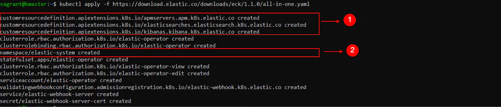
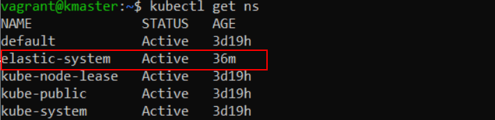
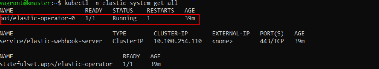
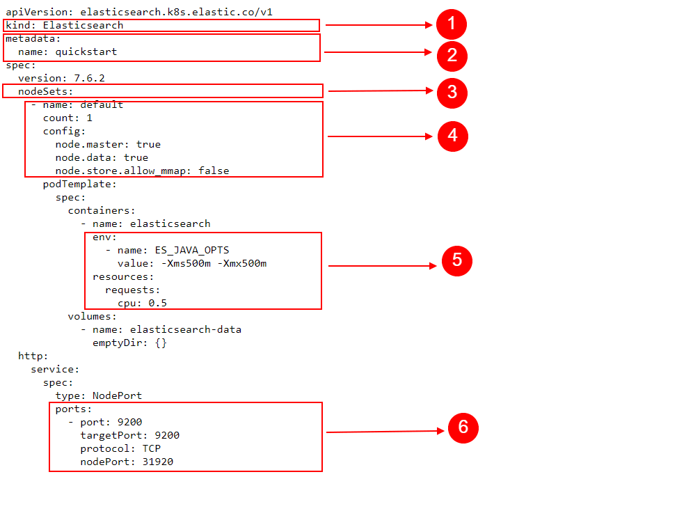
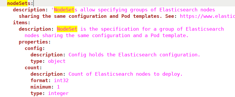
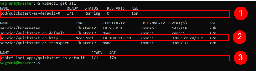
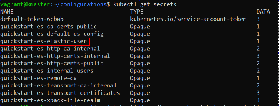
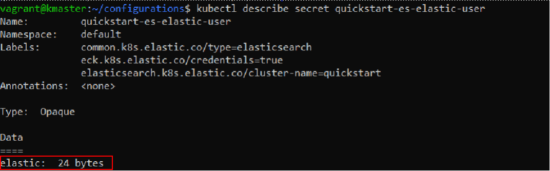
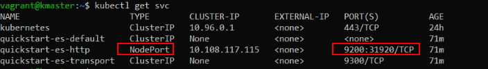
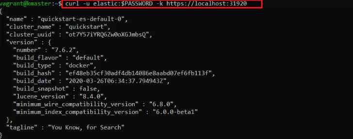
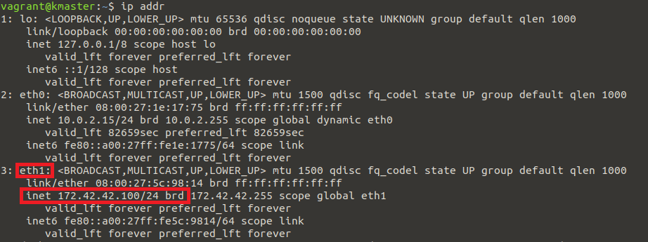
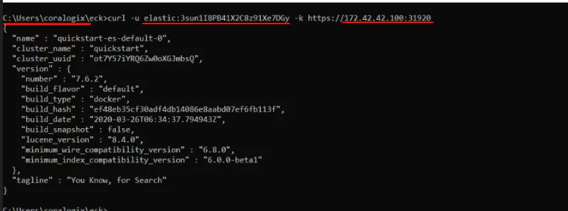
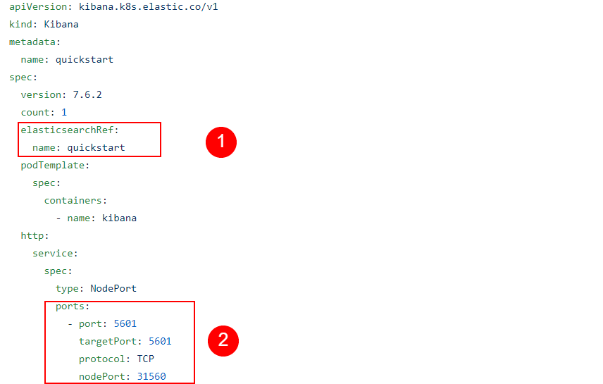
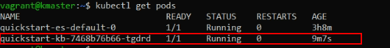
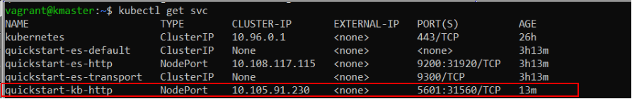
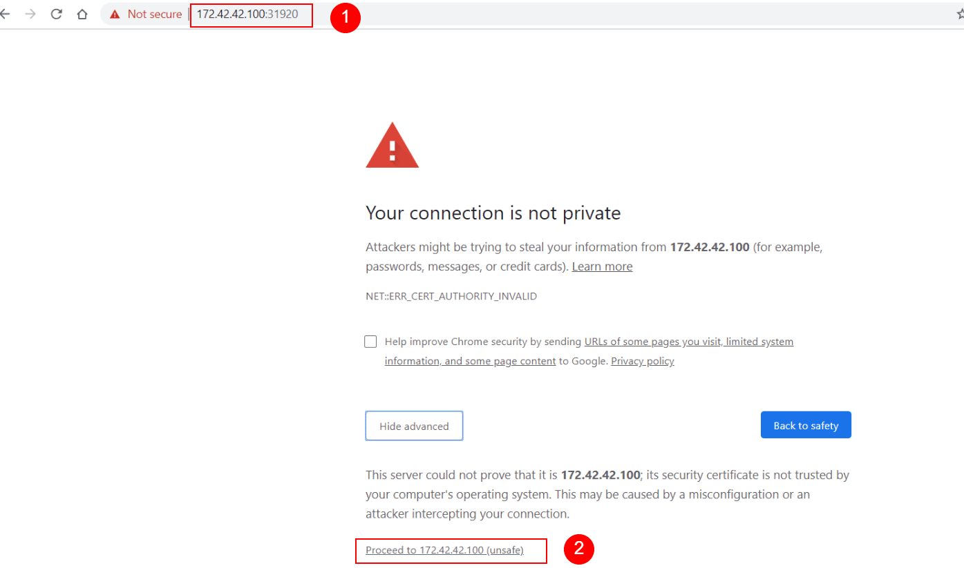
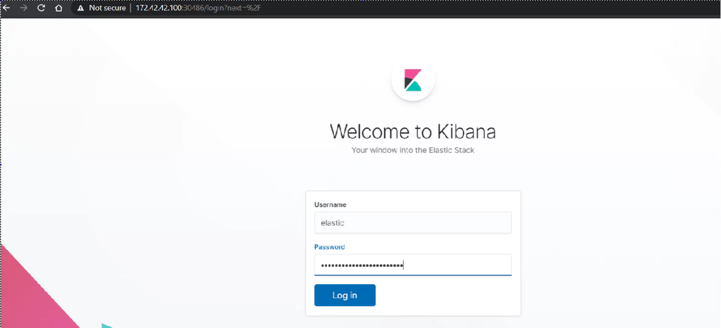
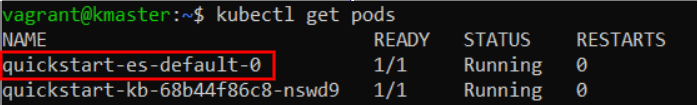
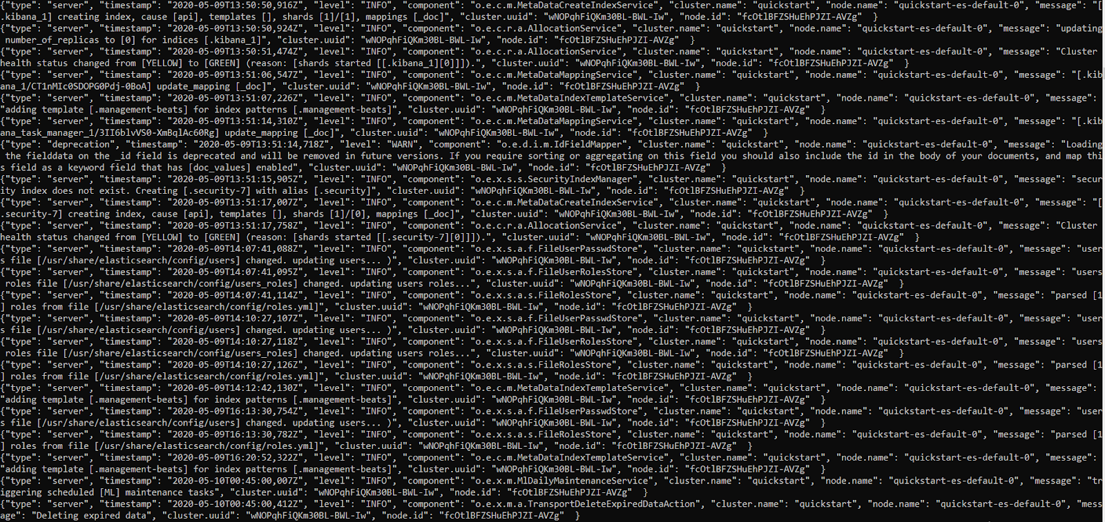
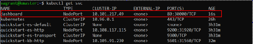
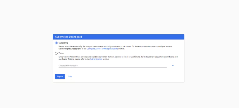
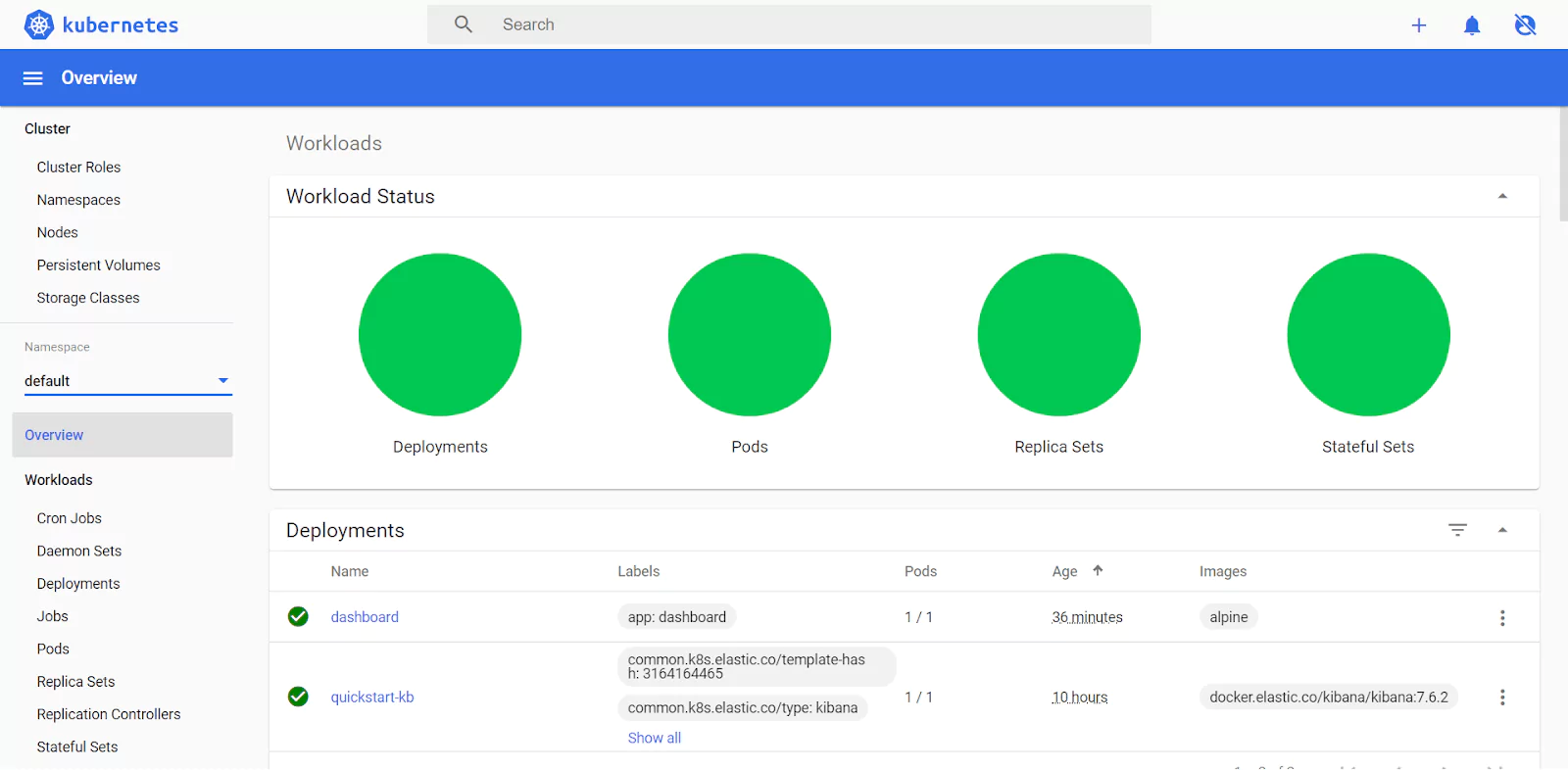
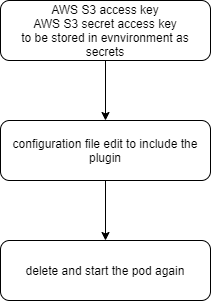

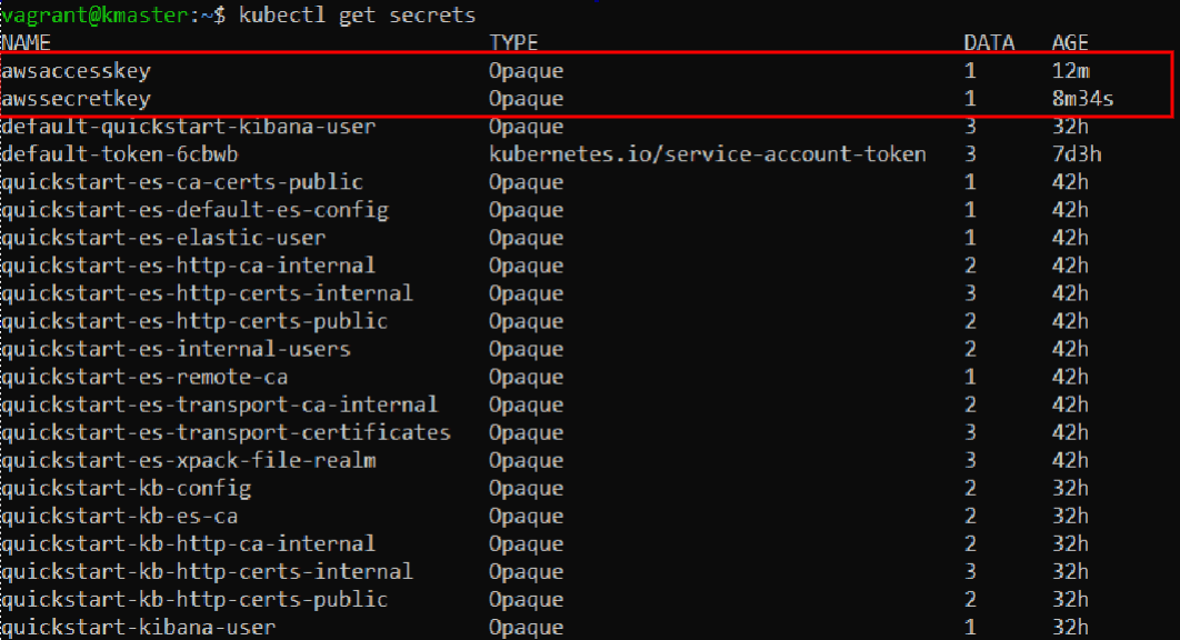
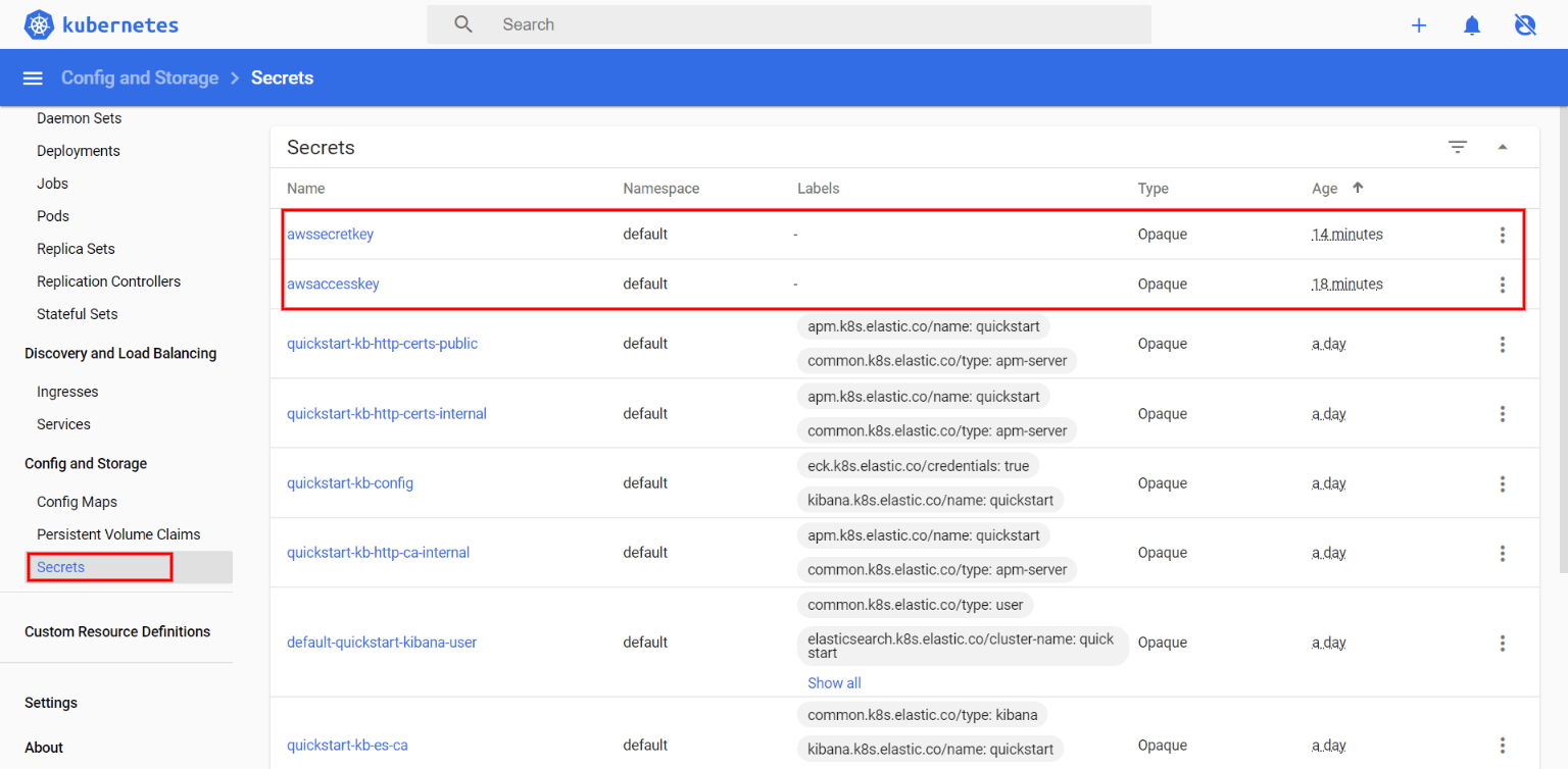
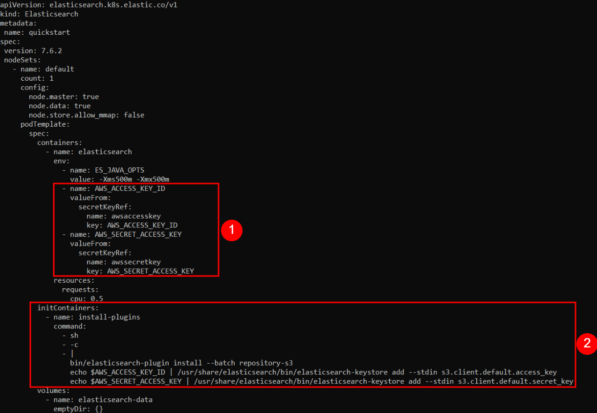
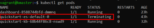
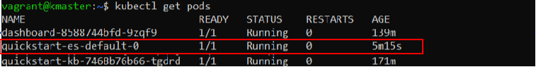
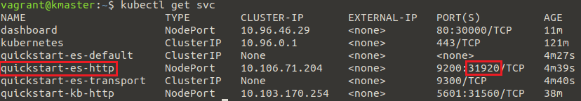
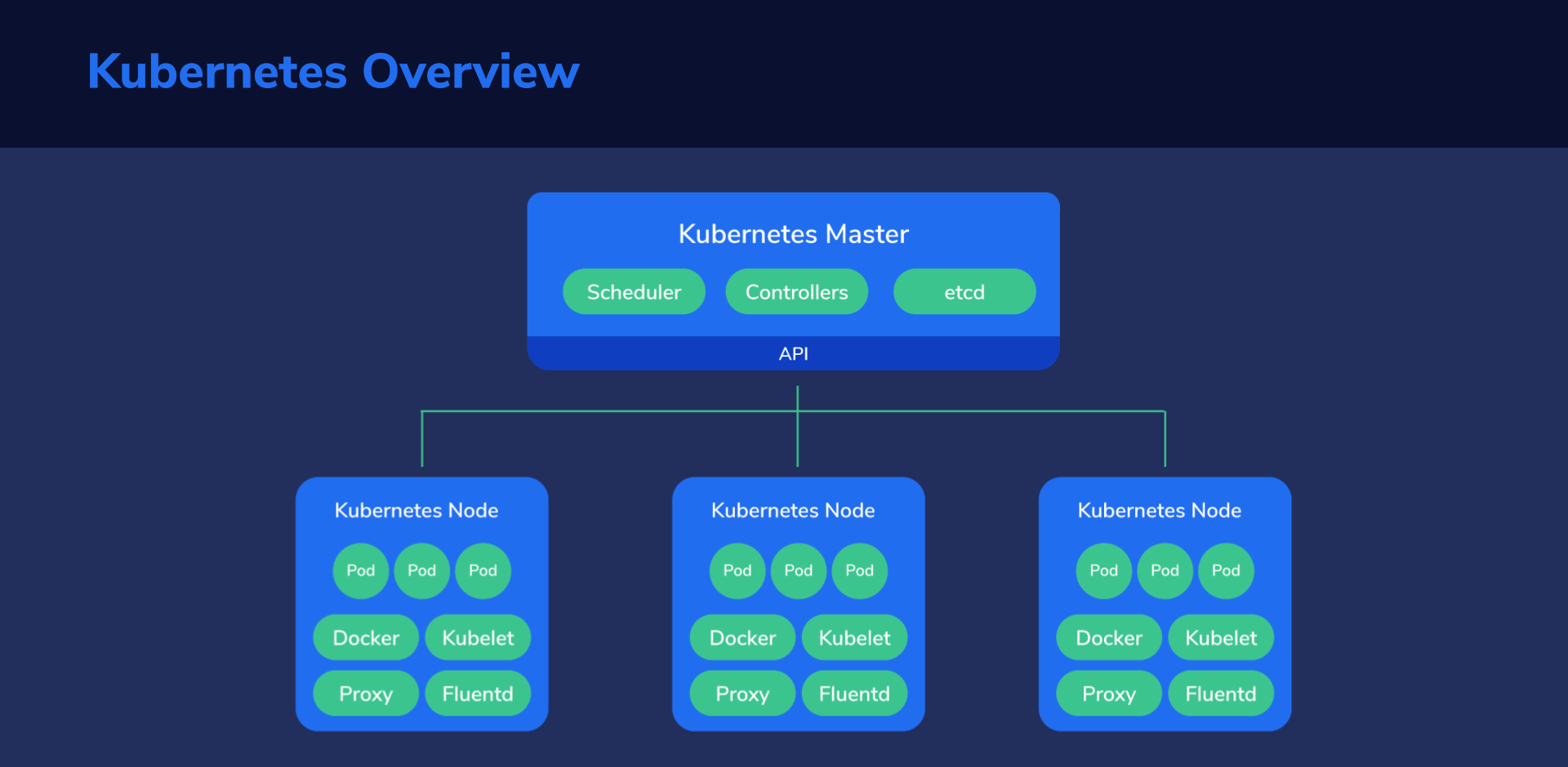
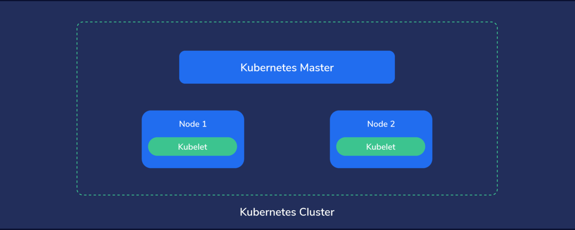
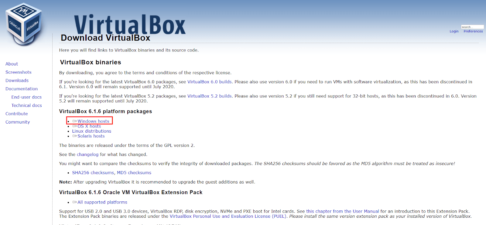
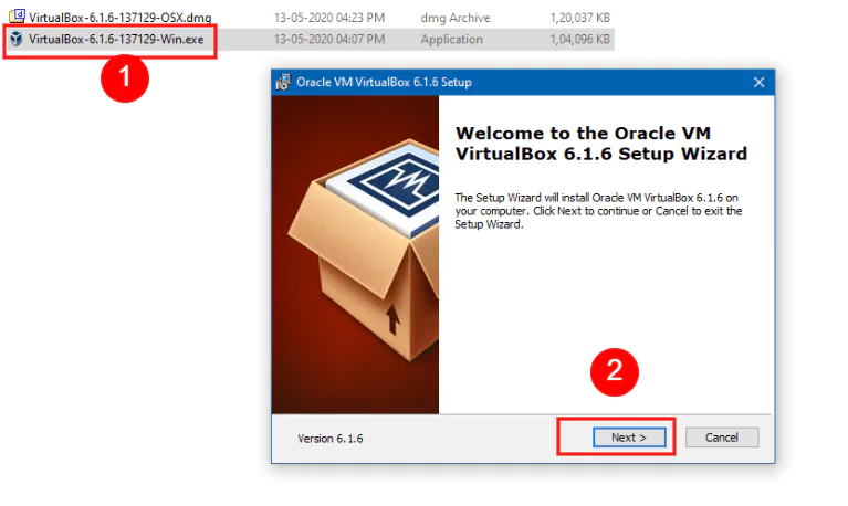
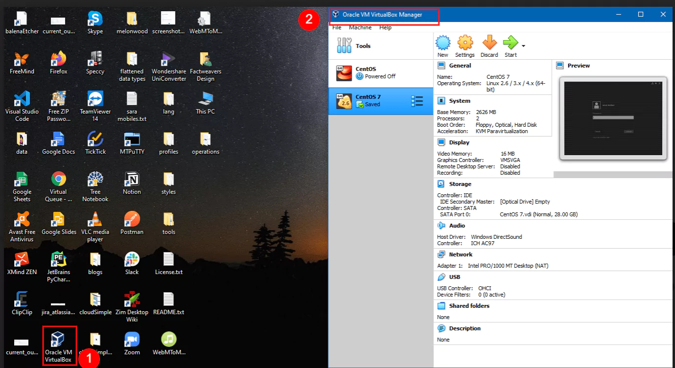
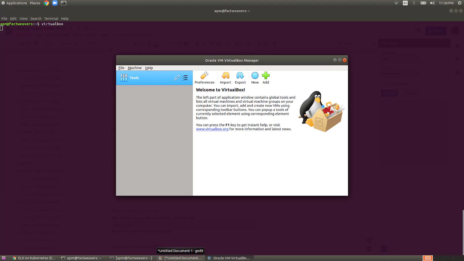
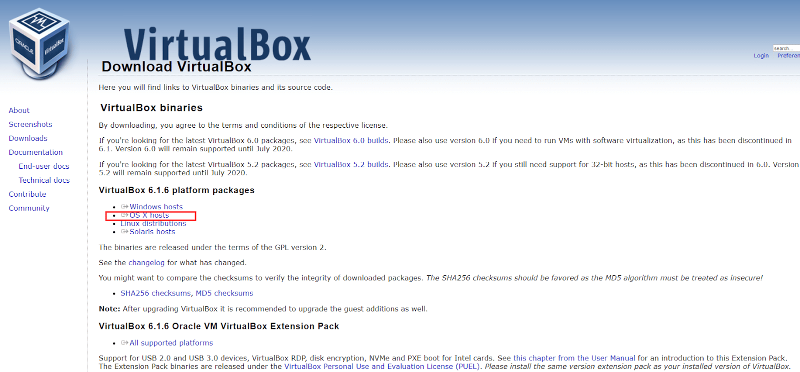
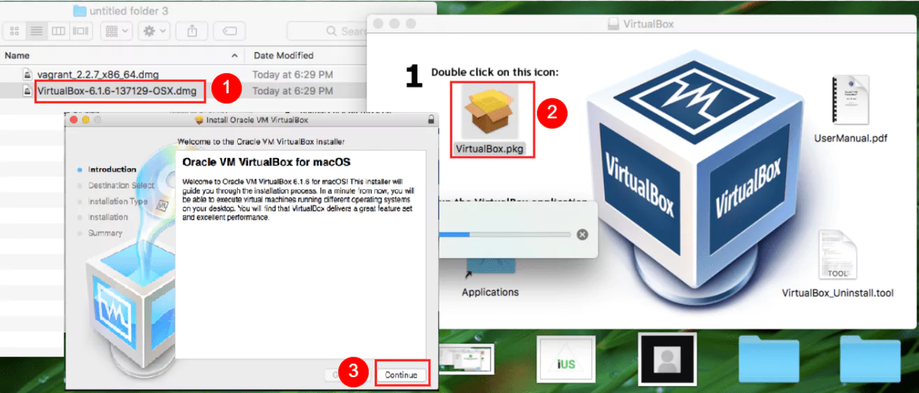
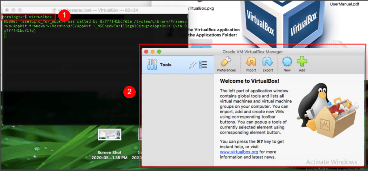
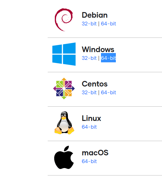
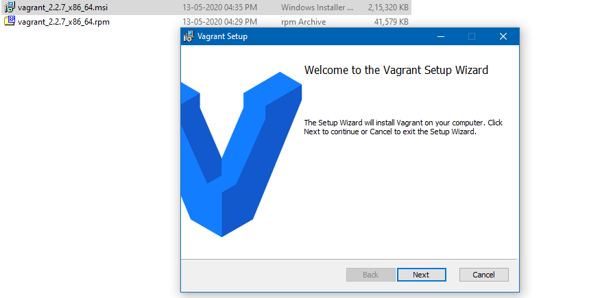

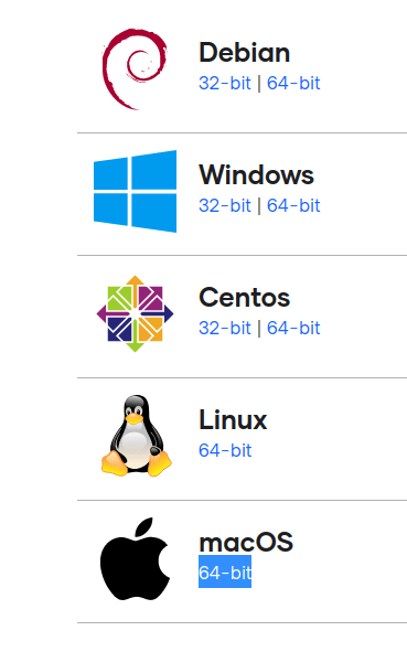
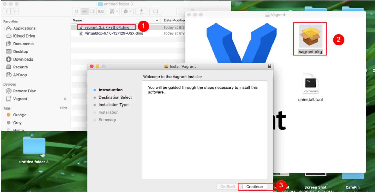
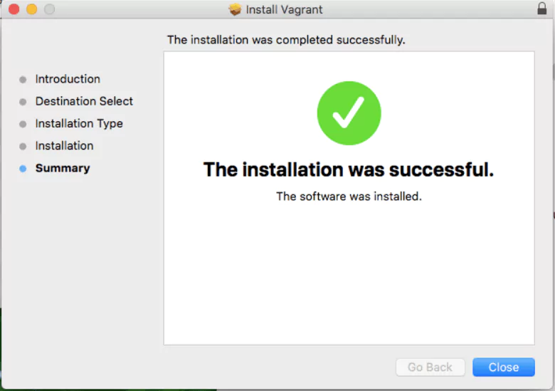
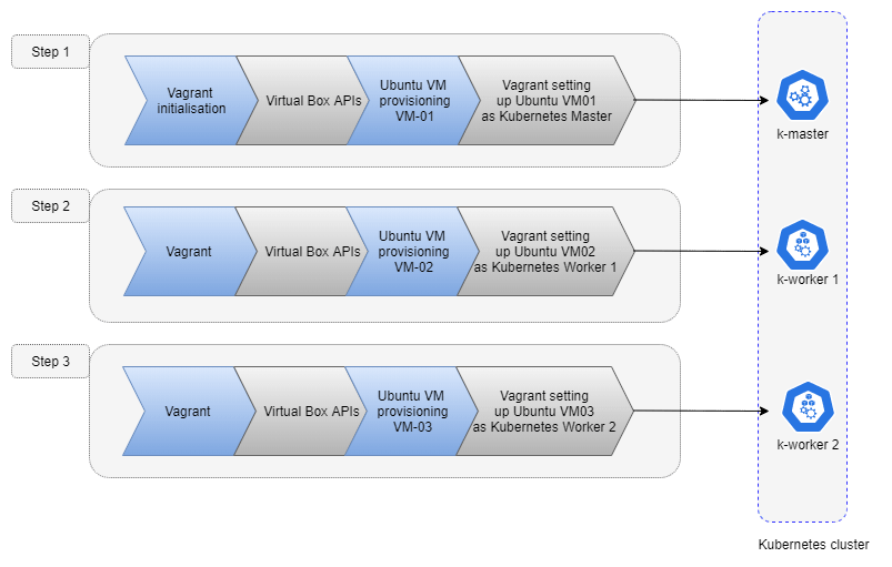
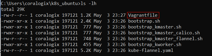
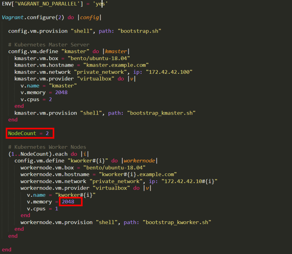
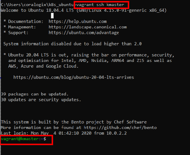
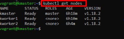

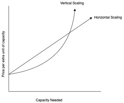
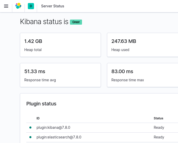
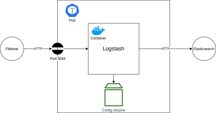
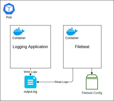
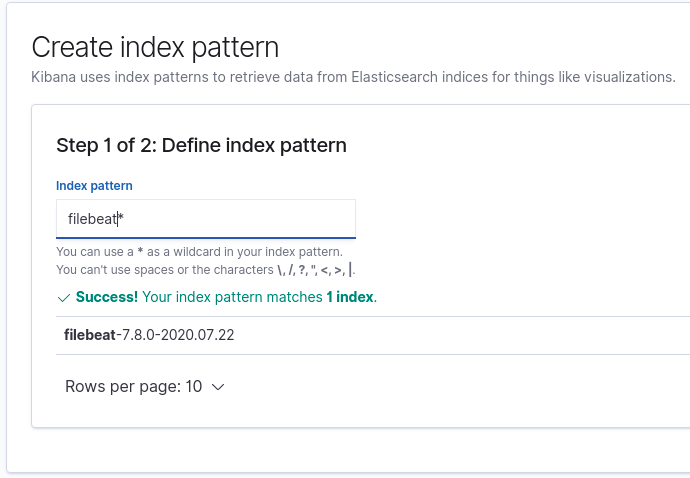
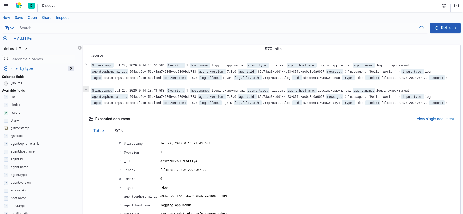


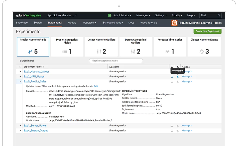
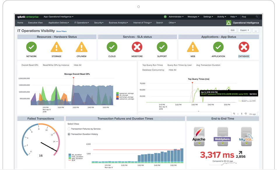
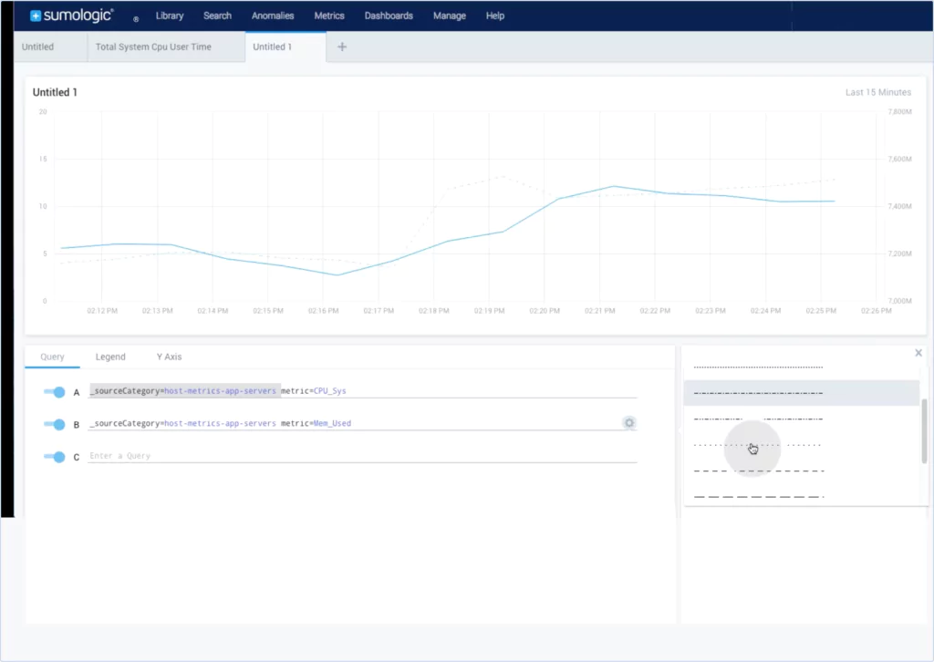
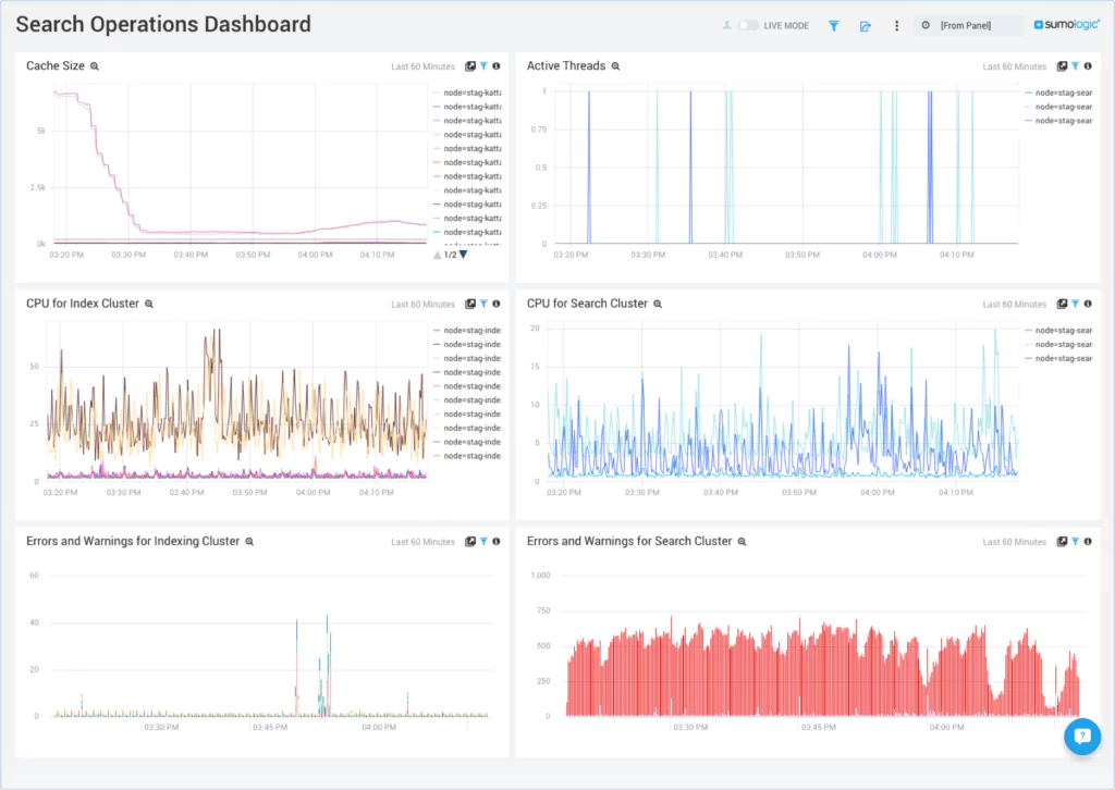
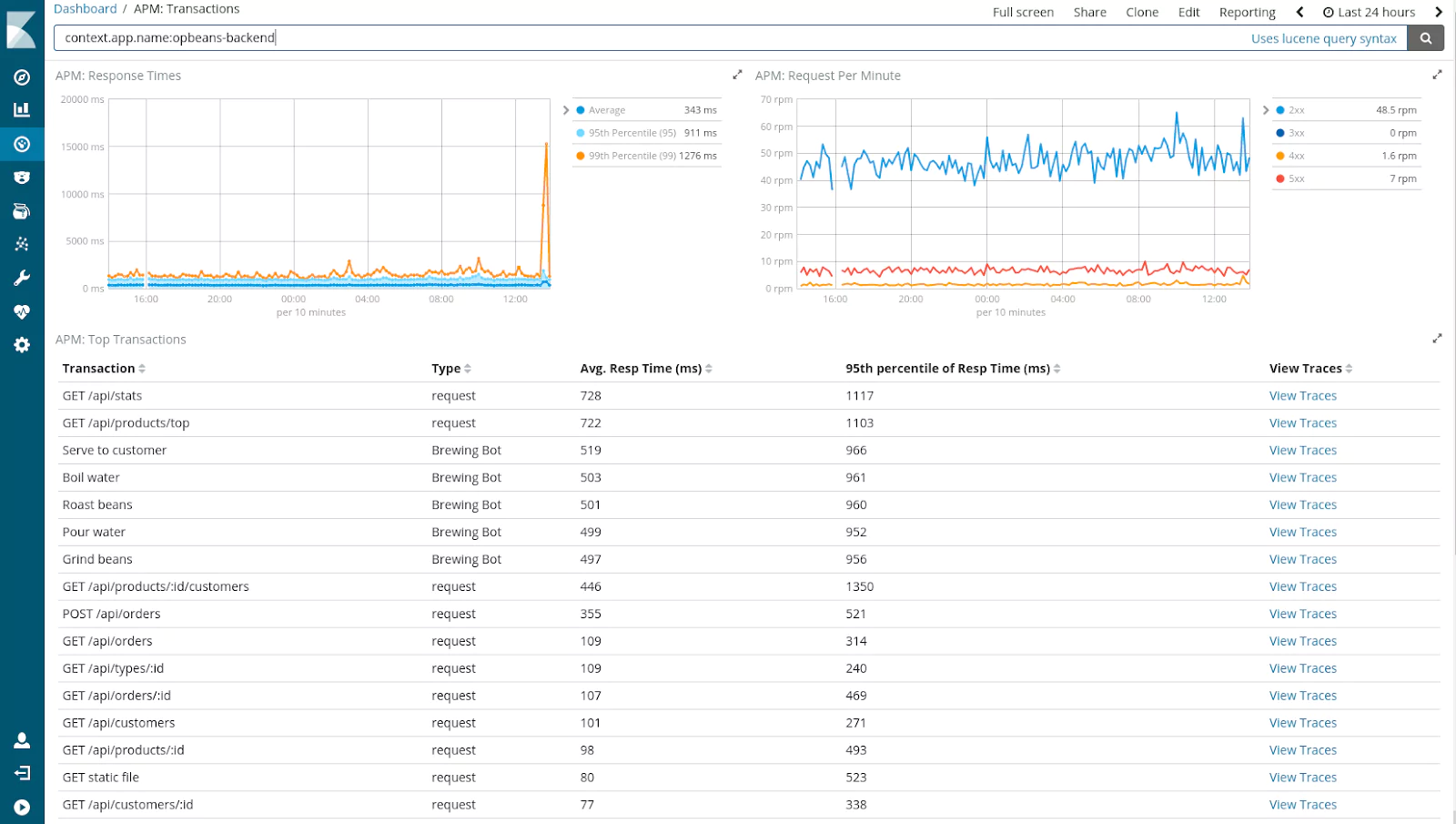
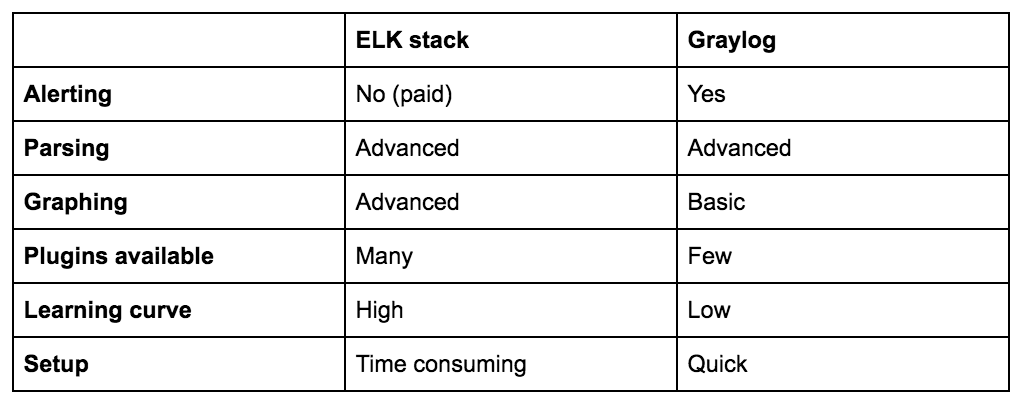

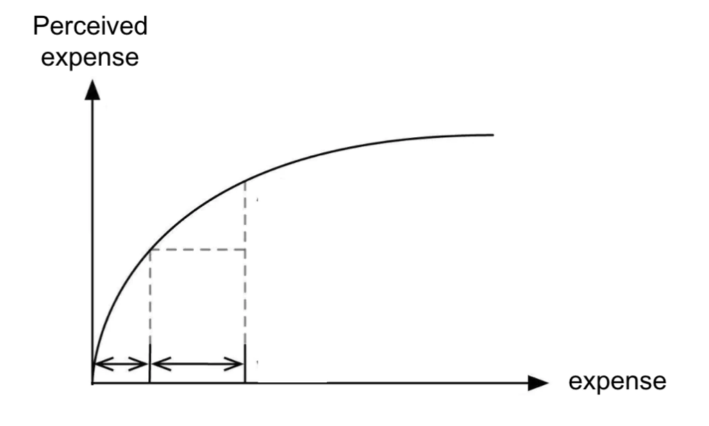
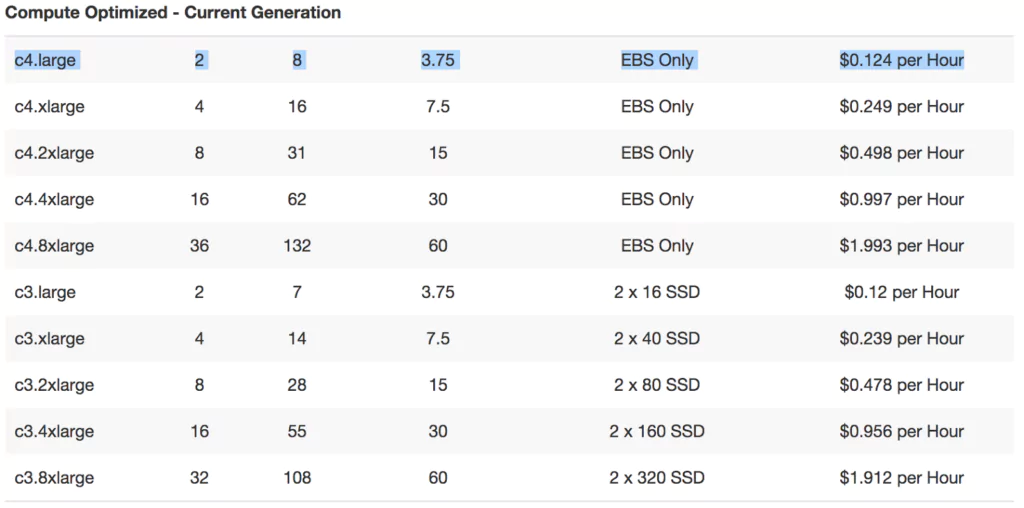
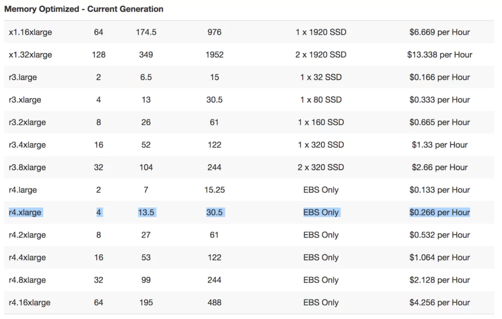
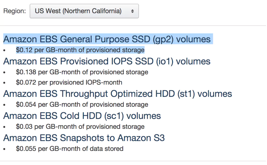
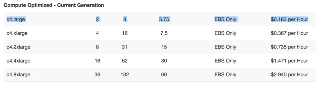
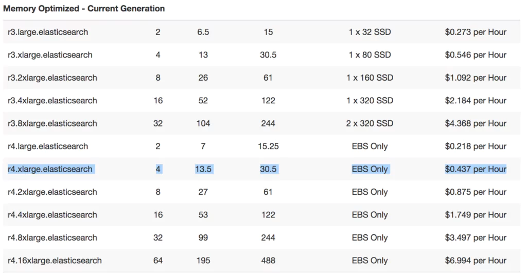
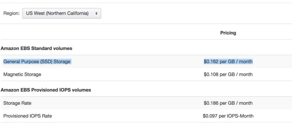