Amid a big data boom, more and more information is being generated from various sources at staggering rates. But without the proper metrics for your data, businesses with large quantities of information may find it challenging to effectively and grow in competitive markets.
For example, high-quality data lets you make informed decisions that are based on derived insights, enhance customer experiences, and drive sustainable growth. On the other hand, poor data quality can set companies back an average of $12.9 million annually, according to Gartner. To help you improve your company’s data quality and drive higher return on investment, we’ll go over what data quality metrics are and offer pro-tips on optimizing your own metrics.
What are data quality metrics?
A measurement system needs to be used to rank data quality. Data quality metrics are key performance indicators (KPIs) that indicate data is healthy and ready to be used. Data observability standards use six metrics that demonstrate data quality. The metrics include:
Accuracy
Accuracy measures whether data conveys true information or not. Ask yourself, does the data reflect reality accurately and factually?
Completeness
Your data should contain all information needed to serve its intended purpose, which could vary from sending an email to a list of customers to a complex analysis of last year’s sales.
Consistency
Different databases may measure the same information but record different values. Does your data differ depending on the source?
Timeliness or currency
Timeliness measures the age of data. The more current the data is, the more likely the information is to be accurate and relevant. Timeliness also requires timestamps to be recorded with all data.
Uniqueness
Uniqueness checks for duplicates in a data set. Duplicates can skew analytics, so any found should be merged or removed.
Validity or uniformity
Validity measures whether or not data is presented in the same format. Data should have proper types, and the data format should be consistent for analysis.
5 tips to optimize data quality metrics
Data collected and stored should meet quality standards to be trusted and used meaningfully. Data quality standards should also take subjective definitions of quality that apply to your company and data set in order to convert them into qualitative values that indicate data health.
Below are expert tips to help understand what to prioritize when generating and using data quality metrics:
Let use-cases drive data quality metrics
Design your data quality metrics using the understanding of what data in your company is used for. For example, data may be used in gaming to customize a user’s in-game experience.
Data could also be used to drive ad campaigns for new in-game features. Write down use cases that connect data quality metrics to their ultimate goals. This will help developers understand why specific data quality metrics are important, and what tolerances may be applied to them.
Data quality metrics may also link to other metrics already recorded in your observability platform. Link data quality metrics to use cases and marketing metrics to measure outcomes resulting from data usage quantitatively.
Identify pain points
After use cases are identified, a list of valuable metrics to generate can be prioritized based on which has been the most troublesome. Ask yourself the following questions, have game user’s not responded as well as expected to recently launched features? Have users complained about a game experience that data showed they would likely enjoy?
Look at the data associated with these use cases first. If no data metrics exist, generate these before other, more stable, data is reviewed. If metrics do already exist, check them to see if there were data issues present that would have affected stakeholders’ decisions. Use results to drive better metrics, alerting, and data quality.
Implement data profiling and cleansing
Data profiling involves analyzing data to identify anomalies, inconsistencies, or missing values. Use data profiling in conjunction with data quality metrics to gain insights into the quality of your data in real time and identify areas that need improvement.
After profiling, if necessary, perform data cleansing to address issues such as duplicate records, missing values, and incorrect entries. Regularly scheduled data cleansing routines help maintain data accuracy. Data cleansing can also be run whenever data corruption reaches some threshold level.
Be aware that profiling and cleansing data both may take significant memory. Ensure memory usage is kept within required limits by monitoring data usage while performing these tasks.
Continuously monitor metrics
Monitor data quality metrics to identify trends, patterns, and potential issues. Define key performance indicators (KPIs) related to data quality and track them regularly.
Set up alerts or notifications to flag potential data quality problems as soon as they arise so that action can be taken promptly. Regularly reviewing data quality metrics allows you to identify areas of improvement and make necessary adjustments to maintain high data quality standards.
Make metrics actionable
Data quality metrics and KPIs must be created and displayed so actions can be easily seen and taken. Up-to-date metrics should always be available for viewing on the Coralogix custom dashboard configured in a way that can be easily understood by data engineers, developers, and stakeholders alike. (You should be able to see the data health status at a glance to know if actions should be taken to fix anything.)
Each metric should be displayed based on its usefulness. The timeliness metric measuring how old data is should be updated periodically to indicate the current age of data. When data becomes too old, action should be taken to update or remove expired data. The Coralogix custom webhooks alert could be used to trigger automatic actions wherever available.
In a rapidly evolving realm of IT, organizations are constantly seeking peak performance and dependability, leading them to rely on a full stack observability platform to obtain valuable system insights.
That’s why the topic of logs vs metrics is so important with both of these data sources playing a vital role, as any full-stack observability guide would tell you, serving as essential elements for efficient system monitoring and troubleshooting. But what are logs and metrics, exactly?
In this article, we’ll take a closer look at logs vs metrics, explore their differences, and see how they can work together to achieve even better results.
What are logs?
Logs serve as a detailed record of events and activities within a system. They provide a chronological narrative of what happens in the system, enabling teams to gain visibility into the inner workings of applications, servers, and networks.
Log messages can contain information about user authentication, database queries, or error messages. They can present different levels, for instance:
Information for every action that was successful, like a server start.
Debug for information that is useful in a development environment, but rarely in production
Warning, which is slightly less severe than errors, signaling that something might fail in the future if no action is taken
Error when something has gone wrong and a failure has been detected in the system.
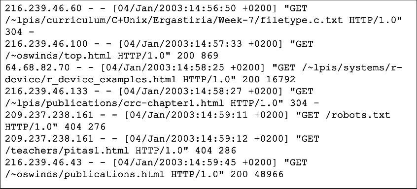
Logs usually take the form of unstructured text with a timestamp:
Logs offer numerous benefits. They are crucial during troubleshooting to diagnose issues and identify the root cause of problems. By analyzing logs, IT professionals and DevOps teams can gain valuable insights into system behavior and quickly resolve issues.
Logs also play a vital role in meeting regulatory requirements and ensuring system security. They offer a comprehensive audit trail, enabling organizations to track and monitor user activities, identify potential security breaches, and maintain compliance with industry standards. They also provide a wealth of performance-related information, allowing teams to monitor system behavior, track response times, identify bottlenecks, and optimize performance.
Despite their many advantages, working with logs can present certain challenges. Logs often generate massive volumes of data, making it difficult to filter through and extract the relevant information. It is also important to note that logs don’t always have the same structure and format, which means that developers need to set up specific parsing and filtering capabilities.
What are metrics?
Metrics, on the other hand, provide a more aggregated and high-level view of system performance. They offer quantifiable measurements and statistical data, providing insights into overall system health, capacity, and usage. Examples of metrics include measurements such as response time, error rate, request throughput, and CPU usage.
Metrics offer several benefits, including:
Real-time monitoring: Metrics provide continuous monitoring capabilities, allowing teams to gain immediate insights into system performance and detect anomalies in real time. This enables proactive troubleshooting and rapid response to potential issues.
Scalability and capacity planning: Metrics help organizations understand system capacity and scalability needs. By monitoring key metrics such as CPU utilization, memory usage, and network throughput, teams can make informed decisions about resource allocation and ensure optimal performance.
Trend analysis: Metrics provide historical data that can be analyzed to identify patterns and trends. This information can be invaluable for capacity planning, forecasting, and identifying long-term performance trends.
While metrics offer significant advantages, they also have limitations. Metrics provide aggregated data, which means that detailed event-level information may be lost. Additionally, some complex system behaviors and edge cases may not be captured effectively through metrics alone.
Logs vs metrics: Do I need both?
The decision to use both metrics and logs depends on the specific requirements of your organization. In many cases, leveraging both logs and metrics is highly recommended, as they complement each other and provide a holistic view of system behavior. While metrics offer a high-level overview of system performance and health, logs provide the necessary context and details for in-depth analysis.
Let’s say you’re a site reliability engineer responsible for maintaining a large e-commerce platform. You have a set of metrics in place to monitor key performance indicators such as response time, error rate, and transaction throughput.
While analyzing the metrics, you notice a sudden increase in the error rate for the checkout process. The error rate metric shows a significant spike, indicating that a problem has occurred. This metric alerts you to the presence of an issue that needs investigation.
To investigate the root cause of the increased error rate, you turn to the logs associated with the checkout process. These logs contain detailed information about each step of the checkout flow, including customer interactions, API calls, and system responses.
By examining the logs during the time period of the increased error rate, you can pinpoint the specific errors and related events that contributed to the problem. You may discover that a new version of a payment gateway integration was deployed during that time, causing compatibility issues with the existing system.
The logs might reveal errors related to failed API calls, timeouts, or incorrect data formats. Armed with the insights gained from the logs, you can take appropriate actions to resolve the issue. In this example, you might roll back the problematic payment gateway integration to a previous version or collaborate with the development team to fix the compatibility issues.
After implementing the necessary changes, you can monitor both metrics and logs to ensure that the error rate returns to normal and the checkout process functions smoothly.
Using metrics and logs with Coralogix
Coralogix is a powerful observability platform that offers full-stack observability capabilities, combining metrics and logs in a unified interface. With Coralogix, IT professionals can effortlessly collect, analyze, and visualize both metrics and logs, gaining deep insights into system performance.
By integrating with Coralogix, you can benefit from its advanced log parsing and analysis features, as well as its ability to extract metrics from logs. You can aggregate and visualize logs in real-time, making it easier to spot patterns, anomalies, and potential issues.
Additionally, Coralogix allows you to define custom metrics and key performance indicators (KPIs) based on the extracted data from logs. This combination of metrics and logs enables you to gain comprehensive insights into your system’s behavior, efficiently identify the root causes of problems, and make data-driven decisions for optimizing performance and maintaining robustness in your applications.
Scrum metrics and data observability are an essential indicator of your team’s progress. In an agile team, they help you understand the pace and progress of every sprint, ascertain whether you’re on track for timely delivery or not, and more.
Although scrum metrics are essential, they are only one facet of the delivery process — sure, they ensure you’re on track, but how do you ensure that there are no roadblocks during development?
That’s precisely where observability helps. Observability gives you a granular overview of your application. It monitors and records performance logs continuously, helping you isolate and fix issues before scrum metrics are affected. Using observability makes your scrum team more efficient — let’s see how.
Scrum Metrics: The Current Issues & How Observability Helps
Problem #1:
Imagine a scenario where you’ve just pushed new code into production and see an error. If it’s a single application, you only have to see the logs to pinpoint exactly where the issue lies. However, when you add distributed systems and cloud services to the mix, the cause of the defect can range from a possible server outage to cloud services being down.
Cue the brain-racking deep dives into logs and traces on multiple servers, with everyone from the developers to DevOps engineers doing their testing and mock runs to figure out the what and where.
This is an absolute waste of time because looking at these individually is like hoping to hit the jackpot – you’re lucky if one of you finds it early on, or you might end up clueless for days on end. And not to mention, scrum metrics would be severely impacted the longer this goes on, causing more pressure from clients and product managers.
How observability fixes it:
With observability, you do not need to comb through individual logs and traces — you can track your applications and view real-time data in a centralized dashboard.
Finding where the problem lies becomes as simple as understanding which request is breaking through a system trace. Since observability tools are configured to your entire system, that just means clicking a few buttons to start the process. Further, application observability metrics can help you understand your system uptime, response time, the number of requests per second, and how much processing power or memory an application uses — thereby helping you find the problem quickly.
Thus, you mitigate downtime risks and can even solve issues proactively through triggered alerts.
Problem #2: Hierarchy & Information Sharing
Working in teams is more than distributing tasks and ensuring their timely completion. Information sharing and prompt communication across the ladder are critical to reducing the mean response time to threats. However, if your team prefers individual-level monitoring and problem-solving, they may not readily share or access information as and when required.
This could create a siloed workplace environment where multiple analytics and monitoring tools are used across the board. This purpose-driven approach inhibits any availability of unified metric data and limits information sharing.
How observability fixes it:
Observability introduces centralized dashboards that enable teams to work on issues collaboratively. You can access pre-formatted, pre-grouped, and segregated logs and traces that indicate defects. A centralized view of these logs simplifies data sharing and coordination within the team, fostering problem-solving through quick communication and teamwork.
Log management tools such as Coralogix’sfull-stack observability platform can generate intelligent reports that help you improve scrum metrics and non-scrum KPIs. Standardizing log formats and traces helps ease the defect and threat-finding process. And your teams can directly access metrics that showcase application health across the organization without compromising on the security of your data.
Let’s look at standard scrum metrics and how observability helps them.
Scrum Metrics & How Observability Improves Them
Sprint Burndown
Sprint burndown is one of the most common scrum metrics. It gives information about the tasks completed and tasks remaining. This helps identify whether the team is on track for each sprint.
As the sprints go on and the scheduled production dates draw close, the code gets more complicated and harder to maintain. More importantly, it becomes harder to discern for those not involved in developing bits.
Observability enables fixing the issues early on. With observability, you get a centralized, real-time logging and tracing system that can predictively analyze and group errors, defects, or vulnerabilities. Metrics allow you to monitor your applications in real time and get a holistic view of system performance.
Thus, the effect on your sprint burndown graph is minimal, with significant defects caught beforehand. Observability generates a more balanced sprint burndown graph that shows the exact work done, including fixing defects.
Team Satisfaction
Observability enables easy collaboration, and information sharing, and gives an overview of how the system performs in real time. A comprehensive centralized observability platform allows developers to analyze logs quickly, fix defects easily, and save the headache of monitoring applications themselves through metrics. And then, they can focus on the job they signed up for — development.
Software Quality
Not all metrics in scrum are easy to measure, and software quality is one of the hardest. The definition is subjective; the closest measurable metric is the escaped defects metric. That’s perhaps why not everyone considers this, but at the end of the day, a software engineering team’s goal is to build high-quality software.
The quicker you find and squash code bugs and vulnerability threats, the easier it gets to improve overall code quality. You’ll have more time to enhance rather than fix and focus more on writing “good code” instead of “code that works.”
Escaped Defects
Have you ever deployed code that works flawlessly in pre-production but breaks immediately in production? Don’t worry — we’ve all been there!
That’s precisely why the escaped defects metric is a core scrum metric. It gives you a good overview of your software’s performance in production.
Implementing observability can directly improve this metric. A good log management and analytics platform like Coralogix can help you identify most bugs proactively through real-time reporting and alerting systems. This reduces the number of defects you may have missed, thus reducing the escaped defects metric.
You benefit from improved system performance and a reduced overall cost and technical debt.
Defect Density
Defect density goes hand-in-hand with escaped defects, especially for larger projects. It measures the number of defects relative to the size of the project.
You could measure this for a class, a package, a set of classes or packages of that deployment, etc. Observability improves the overall performance here. Since you can monitor and generate centralized logs, you can now analyze the defect density and dive deeper into the “why.” Also, using application metrics, you can figure out individual application performance and how efficiently your system works when they are integrated together.
Typically, this metric is used to study irregular defects and answer questions like “are some parts of the code particularly defective?” or “Are some areas out of analysis coverage?” etc. But with observability, you can answer questions like “what’s causing so many defects in these areas?” as defect density and observability complement each other.
Use Observability To Enhance Scrum Metrics
Monitoring scrum KPIs can help developers make better-informed decisions. But these metrics can be hard to track when it comes to developing and deploying modern, distributed systems and microservices. Often, scrum metrics are impacted due to preventable bugs and coordination issues across teams.
Introducing full observability to your stack can revamp the complete development process, significantly improving many crucial scrum metrics. You get a clear understanding of your application health at all times and reduce costs while boosting team morale. If you’re ready to harness the power of observability, contact Coralogix today!
Alerting has been a fundamental part of operations strategy for the past decade. An entire industry is built around delivering valuable, actionable alerts to engineers and customers as quickly as possible. We will explore what’s missing from your alerts and how Coralogix Flow Alerts solve a fundamental problem in the observability industry.
What does everyone want from their alerts?
When engineers build their alerts, they focus on making them as useful as possible, but how do we define useful? While this is a complicated question, we can break the utility of an alert into a few easy points:
Actionable: The information that the alert gives you is usable, and tells you everything you need to know to respond to the situation, with minimal work on your part to piece together what is going on.
Accurate: Your alerts trigger in the correct situation, and they contain correct information.
Timely: Your alerts tell you, as soon as possible, the information you need, when you need it.
For many engineers, achieving these three qualities is a never-ending battle. Engineers are constantly chasing after the smallest, valuable set of alerts we can possibly have to minimize noise and maximize uptime.
However, one key feature is missing from almost every alerting provider, and it goes right to the heart of observability in 2022.
The biggest blocker to the next stage of alerting
If we host our own solution, perhaps with an ELK stack and Prometheus, as is so common in the industry, we are left with some natural alerting options. Alertmanager integrates nicely with Prometheus, and Kibana comes with its own alerting functionality, so you have everything you need, right? Not quite.
Your observability data has been siloed into two specific datastores: Elasticsearch and Prometheus. As soon as you do this, you introduce an architectural complication.
How would you write an alert around your logs AND your metrics?
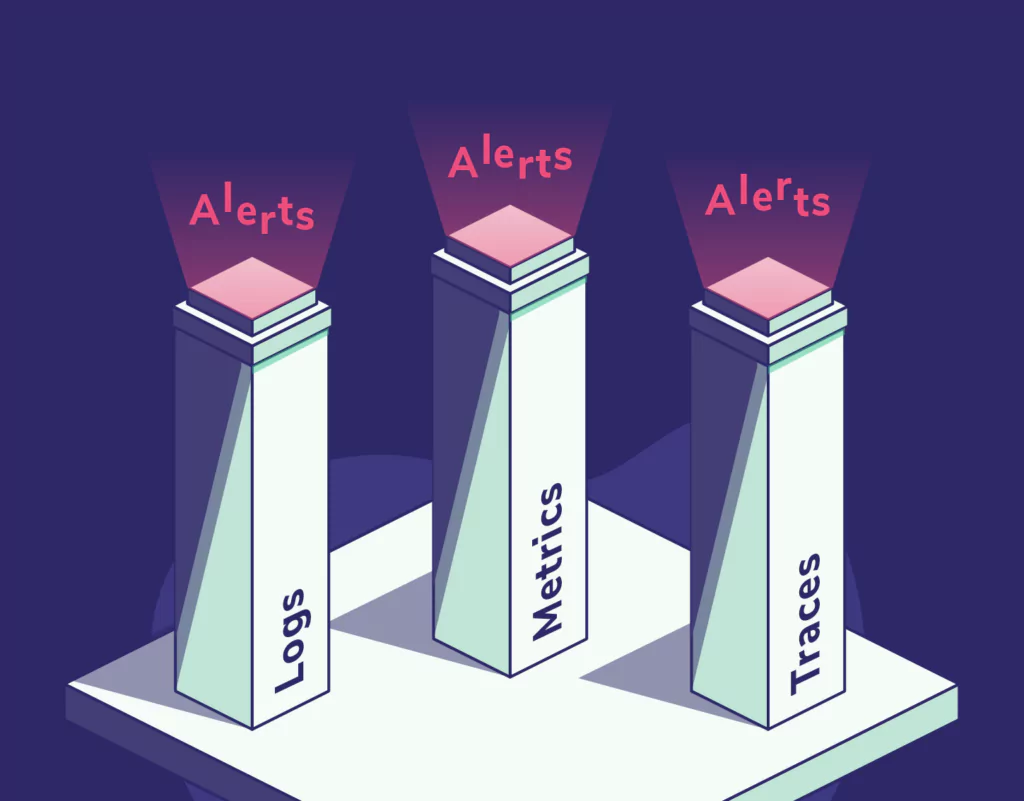
Despite how simple this sounds, this is something that is not supported by the vast majority of SaaS observability providers or open-source tooling. Metrics, logs, and traces are treated as separate pillars, filtering down into our alerting strategies.
It isn’t clear how this came about, but you only need to look at the troubleshooting practices of any engineer to work out that it’s suboptimal. As soon as a metric alert fires, the engineer looks at the logs to verify. As soon as a log alert fires, the engineer looks at the metrics to better understand. It’s clear that all of this data is used for the same purpose, but we silo it off into separate storage solutions and, in doing so, make our life more difficult.
So what can we do?
The answer is twofold. Firstly, we need to bring all of our observability data into a single place, to build a single pane of glass for our system. Aside from alerting, this makes monitoring and general querying more straightforward. It removes the complex learning curve associated with many open-source tools, which speeds up the time it takes for engineers to become familiar with their chosen approach to observability. However, getting data into one place isn’t enough. Your chosen platform needs to support holistic alerting. And there is only one provider on the market – Coralogix.
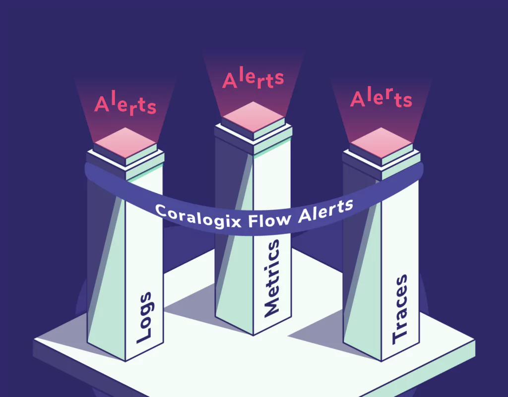
Flow alerts cross the barrier between logs, metrics, and traces
There are many SaaS observability providers out there that will consume your logs, metrics, and traces, but none of them can tie all of this data together into a single, cohesive alert that completely describes an outage, making use of your logs, metrics, and traces in the same alert.
Flow alerts enable you to view your entire system globally without being constrained to a single data type. This brings some key benefits that directly address the great limitations in alerting:
Accurate: With flow alerts, you can track activity across all of your observability data, enabling you to outline precisely the conditions for an incident. This reduces noise because your alerts aren’t too sensitive or based on only part of the data. They’re perfectly calibrated to the behavior of your system.
Actionable: Flow alerts tell you everything that has happened, leading up to an incident, not just the incident itself. This gives you all of the information you need, in one place, to remedy an outage, without hunting for associated data in your logs or metrics.
Timely: Flow alerts are processed within our Streama technology, meaning your alerts are processed and actioned in-stream, rather than waiting for expensive I/O and database operations to complete.
Like cloud-native and DevOps, full-stack observability is one of those software development terms that can sound like an empty buzzword. Look past the jargon, and you’ll find considerable value to be unlocked from building data observability into each layer of your software stack.
Before we get into the details of monitoring observability, let’s take a moment to discuss the context. Over the last two decades, software development and architecture trends have departed from single-stack, monolithic designs toward distributed, containerized deployments that can leverage the benefits of cloud-hosted, serverless infrastructure.
This provides a range of benefits, but it also creates a more complex landscape to maintain and manage: software breaks down into smaller, independent services that deploy to a mix of virtual machines and containers hosted both on-site and in the cloud, with additional layers of software required to manage automatic scaling and updates to each service, as well as connectivity between services.
At the same time, the industry has seen a shift from the traditional linear build-test-deploy model to a more iterative methodology that blurs the boundaries between software development and operations. This DevOps approach has two main elements.
First, developers have more visibility and responsibility for their code’s performance once released. Second, operations teams are getting involved in the earlier stages of development — defining infrastructure with code, building in shorter feedback loops, and working with developers to instrument code so that it can output signals about how it’s behaving once released.
With richer insights into a system’s performance, developers can investigate issues more efficiently, make better coding decisions, and deploy changes faster.
Observability closely ties into the DevOps philosophy: it plays a central role in providing the insights that inform developers’ decisions. It depends on addressing matters traditionally owned by ops teams earlier in the development process.
What is full-stack observability?
Unlike monitoring, observability is not what you do. Instead, it’s a quality or property of a software system. A system is observable if you can ask questions about the data it emits to gain insight into how it behaves. Whereas monitoring focuses on a pre-determined set of questions — such as how many orders are completed or how many login attempts failed — with an observable system, you don’t need to define the question.
Instead, observability means that enough data is collected upfront allowing you to investigate failures and gain insights into how your software behaves in production, rather than adding extra instrumentation to your code and reproducing the issue.
Once you have built an observable system, you can use the data emitted to monitor the current state and investigate unusual behaviors when they occur. Because the data was already collected, it’s possible to look into what was happening in the lead-up to the issue.
Full-stack observability refers to observability implemented at every layer of the technology stack. – From the containerized infrastructure on which your code is running and the communications between the individual services that make up the system, to the backend database, application logic, and web server that exposes the system to your users.
With full-stack observability, IT teams gain insight into the entire functioning of these complex, distributed systems. Because they can search, analyze, and correlate data from across the entire software stack, they can better understand the relationships and dependencies between the various components. This allows them to maintain systems more effectively, identify and investigate issues quickly, and provide valuable feedback on how the software is used.
So how do you build an observable system? The answer is by instrumenting your code to emit signals and collect telemetry centrally so that you can ask questions about how it’s behaving and why it’s running in production. The types of telemetry can be broken down into what is known as the “four pillars of observability”: metrics, logs, traces, and security data.
Each pillar provides part of the picture, as we’ll discuss in more detail below. Ensuring these types of data are emitted and collating that information into a single observability platform makes it possible to observe how your software behaves and gain insights into its internal workings.
Deriving value from metrics
The first of our four pillars is metrics. These are time series of numbers derived from the system’s behavior. Examples of metrics include the average, minimum, and maximum time taken to respond to requests in the last hour or day, the available memory, or the number of active sessions at a given point in time.
The value of metrics is in indicating your system’s health. You can observe trends and identify any significant changes by plotting metric values over time. For this reason, metrics play a central role in monitoring tools, including those measuring system health (such as disk space, memory, and CPU availability) and those which track application performance (using values such as completed transactions and active users).
While metrics must be derived from raw data, the metrics you want to observe don’t necessarily have to be determined in advance. Part of the art of building an observable system is ensuring that a broad range of data is captured so that you can derive insights from it later; this can include calculating new metrics from the available data.
Gaining specific insights with logs
The next source of telemetry is logs. Logs are time-stamped messages produced by software that record what happened at a given point. Log entries might record a request made to a service, the response served, an error or warning triggered, or an unexpected failure. Logs can be produced from every level of the software stack, including operating systems, container runtimes, service meshes, databases, and application code.
Most software (including IaaS, PaaS, CaaS, SaaS, firewalls, load balancers, reverse proxies, data stores, and streaming platforms) can be configured to emit logs, and any software developed in-house will typically have logging added during development. What causes a log entry to be emitted and the details it includes depend on how the software has been instrumented. This means that the exact format of the log messages and the information they contain will vary across your software stack.
In most cases, log messages are classified using logging levels, which control the amount of information that is output to logs. Enabling a more detailed logging level such as “debug” or “verbose” will generate far more log entries, whereas limiting logging to “warning” or “error” means you’ll only get logs when something goes wrong. If log messages are in a structured format, they can more easily be searched and queried, whereas unstructured logs must be parsed before you can manipulate them programmatically.
Logs’ low-level contextual information makes them helpful in investigating specific issues and failures. For example, you can use logs to determine which requests were produced before a database query ran out of memory or which user accounts accessed a particular file in the last week.
Taken in aggregate, logs can also be analyzed to extrapolate trends and detect past and real-time anomalies (assuming they are processed quickly enough). However, checking the logs from each service in a distributed system is rarely practical. To leverage the benefits of logs, you need to collate them from various sources to a central location so they can be parsed and analyzed in bulk.
Using traces to add context
While metrics provide a high-level indication of your system’s health and logs provide specific details about what was happening at a given time, traces supply the context. Distributed tracing records the chain of events involved in servicing a particular request. This is especially relevant in microservices, where a request triggered by a user or external API call can result in dozens of child requests to different services to formulate the response.
A trace identifies all the child calls related to the initiating request, the order in which they occurred, and the time spent on each one. This makes it much easier to understand how different types of requests flow through a system, so that you can work out where you need to focus your attention and drill down into more detail. For example, suppose you’re trying to locate the source of performance degradation. In that case, traces will help you identify where the most time is being spent on a request so that you can investigate the relevant service in more detail.
Implementing distributed tracing requires code to be instrumented so that trace identifiers are propagated to each child request (known as spans), and the details of each span are forwarded to a database for retrieval and analysis.
Adding security data to the picture
The final element of the observability puzzle is security data. Whereas the first three pillars represent specific types of telemetry, security data refers to a range of data, including network traffic, firewall logs, audit logs and security-related metrics, and information about potential threats and attacks from security monitoring platforms. As a result, security data is both broader and narrower than the first three pillars.
Security data merits inclusion as a pillar in its own right because of the crucial importance of defending against cybersecurity attacks for today’s enterprises. In the same way that the importance of building security into software has been highlighted by the term DevSecOps, including security as a pillar in its own right serves to highlight the role that observability plays in improving software security and the value to be had from bringing all available data into a single platform.
As with metrics, logs, and traces, security data comes from multiple sources. One of the side effects of the trend towards more distributed systems is an increase in the potential attack surface. With application logic and data spread across multiple platforms, the network connections between individual containers and servers and across public and private clouds have become another target for cybercriminals. Collating traffic data from various sources makes it possible to analyze that data more effectively to detect potential threats and investigate issues efficiently.
Using an observability platform
While these four types of telemetry provide valuable data, using each in isolation will not deliver the full benefits of observability. To answer questions about how your system is performing efficiently, you need to bring the data together into a single platform that allows you to make connections between data points and understand the complete picture. This is how an observability platform adds value.
Full-stack observability platforms provide a single source of truth for the state of your system. Rather than logging in to each component of a distributed system to retrieve logs and traces, view metrics, or examine network packets, all the information you need is available from a single location. This saves time and provides you with better context when investigating an issue so that you can get to the source of the problem more quickly.
Armed with a comprehensive picture of how your system behaves at all layers of the software stack, operations teams, software developers, and security specialists can benefit from these insights. Full-stack observability makes it easier for these teams to detect and troubleshoot production issues and monitor changes’ impact as they deploy.
Better visibility of the system’s behavior also reduces the risk associated with trialing and adopting new technologies and platforms, enabling enterprises to move fast without compromising performance, reliability, or security. Finally, having a shared perspective helps to break down siloes and encourages the cross-team collaboration that’s essential to a DevSecOps approach.
Whether it’s Apache, Nginx, ILS, or anything else, web servers are at the core of online services, and web log monitoring and analysis can reveal a treasure trove of information. These logs may be hidden away in many files on disk, split by HTTP status code, timestamp, or agent, among other possibilities. Web access log monitoring is typically analyzed to troubleshoot operational issues, but there is so much more insight that you can draw from this data, from SEO to user experience. Let’s explore what you can do when you really dive into web log analysis.
1. Spotting errors and troubleshooting with web log analysis
Right now, online Internet traffic is exceeding 333 Exabytes per month. This has been growing year on year since the founding of the Internet. With this increase in traffic comes the increased complexity of operational observability. Your web access logs are crucial in the fight to maintain operational excellence. While the details vary, some fields you can expect in all of your web logs include:
Latency
Source IP address
HTTP status code
Resource requested
Request and response size in bytes
These fields are fundamental measures in building a clear picture of your operational excellence. You can use these fields to capture abnormal traffic arriving at your site, which may indicate malicious activity like “bad bot” web scraping. You could also detect an outage in your site by looking at a sudden increase in errors in your HTTP status codes.
2. SEO diagnostics with web logs
68% of online activity begins with a user typing something into a search engine. This means that if you’re not harnessing the power of SEO, you’re potentially missing out on a massive volume of potential traffic and customers. Despite this, almost 90% of content online receives no organic traffic from Google. An SEO-optimized site represents a serious edge in the competitive online market. Web access logs can give you an insight into several key SEO dimensions that will provide you with clear measurements for the success of your SEO campaigns.
42.7% of online users are currently using an ad-blocker, which means that you may see serious disparities between the traffic to your site and the impressions you’re seeing on the PPC ads that you host. Your web log analysis can alert you to this disparity very easily by giving you a clear overall view of the traffic you’re receiving because they are taken on the server-side and don’t depend on the client’s machine to track usage.
You can also verify the IP addresses connected to your site to determine whether Googlebot is scraping and indexing your site. This is crucial because it won’t just tell you if Googlebot is present but also which pages it has accessed, using a combination of the URI field and IP address in your web access logs.
3. Site performance and user experience insights from web log analysis
Your web access logs can also give you insight into how your site performs for your user. This is different from the operational challenge of keeping the site functional and more of a marketing challenge to keep the website snappy, which is vital. Users make decisions about your site in the first 50ms, and if all they see is a white loading page, they’re not going to make favorable conclusions.
The bounce rate increases sharply with increased latency. If your page takes 4 seconds to load, you’ve lost 20% of your potential visitors. Worse, those users will view an average of 3.4 fewer pages than they would if the site took 2 seconds to load. Every second makes a difference.
Your web access logs are the authority on your latency because they tell you the duration of the whole HTTP connection. You can then combine these values with more specific measurements, like the latency of a database query or disk I/O latencies. By optimizing for these values, you can ensure that you’re not losing any of your customers to slow latencies.
Your web access logs may also give you access to the User-Agent header. This header can tell you the browser and operating system that initiated the request. This is essential because it will give you an idea of your customers’ devices and browsers. 52.5% of all online traffic comes from smartphones, so you’re likely missing out if you’re not optimizing for mobile usage.
Wrapping up
Web access log analysis is one of the fundamental pillars of observability; however, the true challenge isn’t simply viewing and analyzing the logs, but in getting all of your observability data into one place to correlate them with one another. Your Nginx logs are powerful, but if you combine them with your other logs, metrics, and traces from CDNs, applications, and more, they form part of an observability tapestry that can yield actionable insights across your entire system.
Quality control and observability of your platform are critical for any customer-facing application. Businesses need to understand their user’s experience in every step of the app or webpage. User engagement can often depend on how well your platform functions, and responding quickly to problems can make a big difference in your application’s success.
AWS monitoring tools can help companies simulate and understand the user experience. It will help alert businesses to issues before they become problems for customers.
The Functionality of AWS Canaries
AWS Canaries are an instantiation of Amazon’s CloudWatch Synthetics. They are configurable scripts that automatically execute to monitor endpoints and APIs. They will follow the flow and perform the actions as real users. The results from the Canary mimic what a real user would see at any given time, allowing teams to validate their customer’s experience.
Tracked metrics using AWS Canaries include availability and latency of your platform’s endpoints and APIs, load time data, and user interface screenshots. They can also monitor linked URLs and website content. AWS Canaries can also check for changes to your endpoint resulting from authorized code changes, phishing, and DDoS attacks.
How AWS Canaries Work
AWS Canaries are scripts that monitor your endpoints and APIs. The scripts follow the same flows that real customers would follow to hit your endpoints. Developers can write Canary scripts using either Node.js or Python, and the scripts run on a headless Google Chrome Browser using Puppeteer for Node.js scripts or Selenium for Python scripts. Canaries run scripts against your platform and log results in one of AWS’s observability tools, such as CloudWatch or XRay. From here, developers can export the data to other tools like Coralogix’s metrics platform for analysis.
AWS Canaries and Observability
AWS Canaries and X-Ray
Developers can set AWS Canaries to use X-Ray for specific runtimes. When X-Ray is enabled, traces indicate latency requests, and the Canaries send failures to X-Ray. These data are explicitly grouped for canary calls, making separating actual calls from AWS Canary calls against your endpoints easier.
Enabling traces can increase the canary’s runtime by up to 7%. Also, set IAM permissions that allow the canary to write to X-Ray.
AWS Canaries and EventBridge
AWS EventBridge can notify various AWS Canary events, including status changes or complete runs. AWS does not guarantee delivery of all Canary events to EventBridge, instead of sending on a best effort basis. Cases where data does not arrive in EventBridge, are expected to be rare.
Canary events can trigger different EventBridge rules and, therefore, different subsequent functions or data transfers to third-party analytics tools. Functions can be written that allow teams to troubleshoot when a canary fails, investigate error states, or monitor workflows.
AWS Canaries and CloudWatch Metrics
AWS Canaries will automatically create Cloudwatch metrics. Metrics published include the percentage of entirely successful and failed canary runs, duration of canary tuns, and the number of responses in the 200, 400, and 500 ranges.
Metrics can be viewed on the CloudWatch Metrics page. They will be present under the CloudWatchSynthetics namespace.
AWS Canaries and Third-Party Analytics
Since AWS Canaries automatically write CloudWatch metrics, metrics streams can be used to deliver data to third-party tools like Coralogix’s scaling metrics platform. CloudWatch metrics streams allow users to send only specific namespaces or all namespaces to third parties. After the stream is created, new metrics will be sent automatically to the third party without limit. AWS does charge based on the number of metrics updates sent.
Creating a Canary
When creating a Canary, developers choose whether to use an AWS-provided blueprint, the inline editor, or import a script from S3. Blueprints provide a simple way to get started with this tool. Developers can create Canaries using several tools such as the Serverless framework, the AWS CLI, or the AWS console. Here we will focus on creating a Canary using a Blueprint with the AWS console.
Create a Canary from the AWS Console
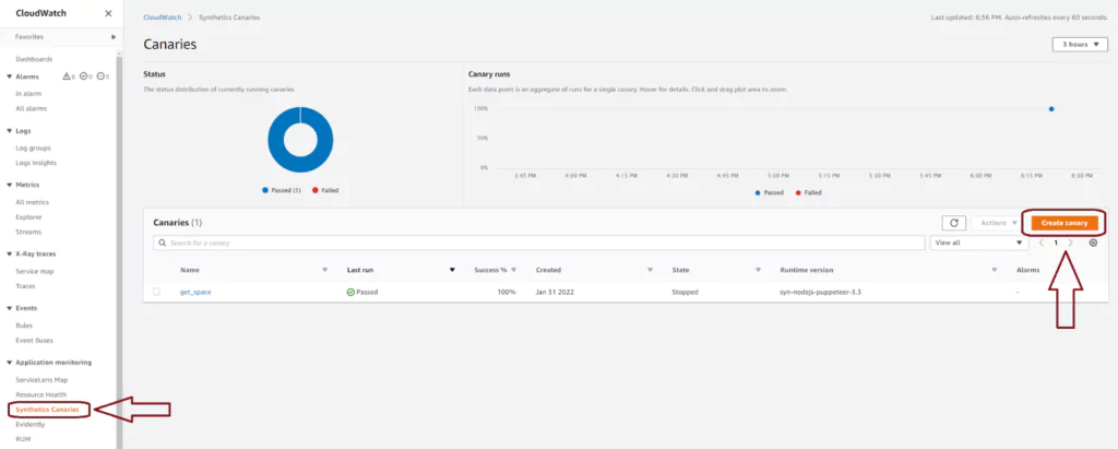
Navigate to the AWS CloudWatch console. You will find Synthetics Canaries in the right-hand menu under the Application monitoring section. This page loads to show you any existing Canaries you have. You can see, at a glance, how many of the most recent runs have passed or failed across all your canaries. You can also select Create canary from this page to make a new AWS Canary and test one of your endpoints.
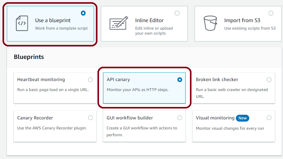
Use a Blueprint to create a Canary quickly
In the first section, you select how to create your new Canary. Here we will choose to use an AWS blueprint, but the inline editor and importing from S3 are also options. There are six blueprints currently available. Each is designed to get developers started on a different common problem. We will use the API canary, which will attempt to call the AWS-deployed API periodically. This option is useful when you want to test an API you own in AWS API Gateway or some other hosted service.
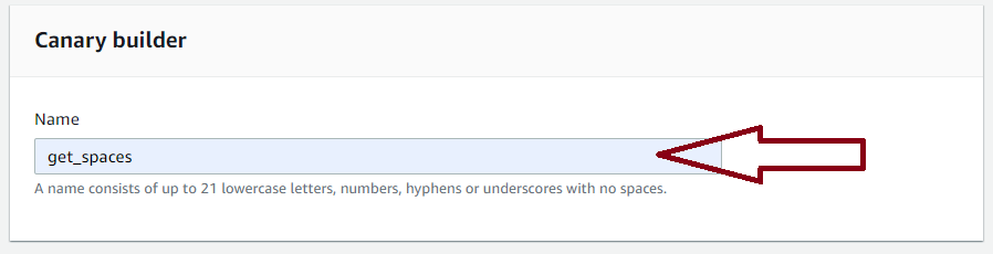
Name your Canary
Next, choose a name for your canary. It does not need to match the name of the API, but this will make it easier to analyze the results if you are testing a large number of endpoints.
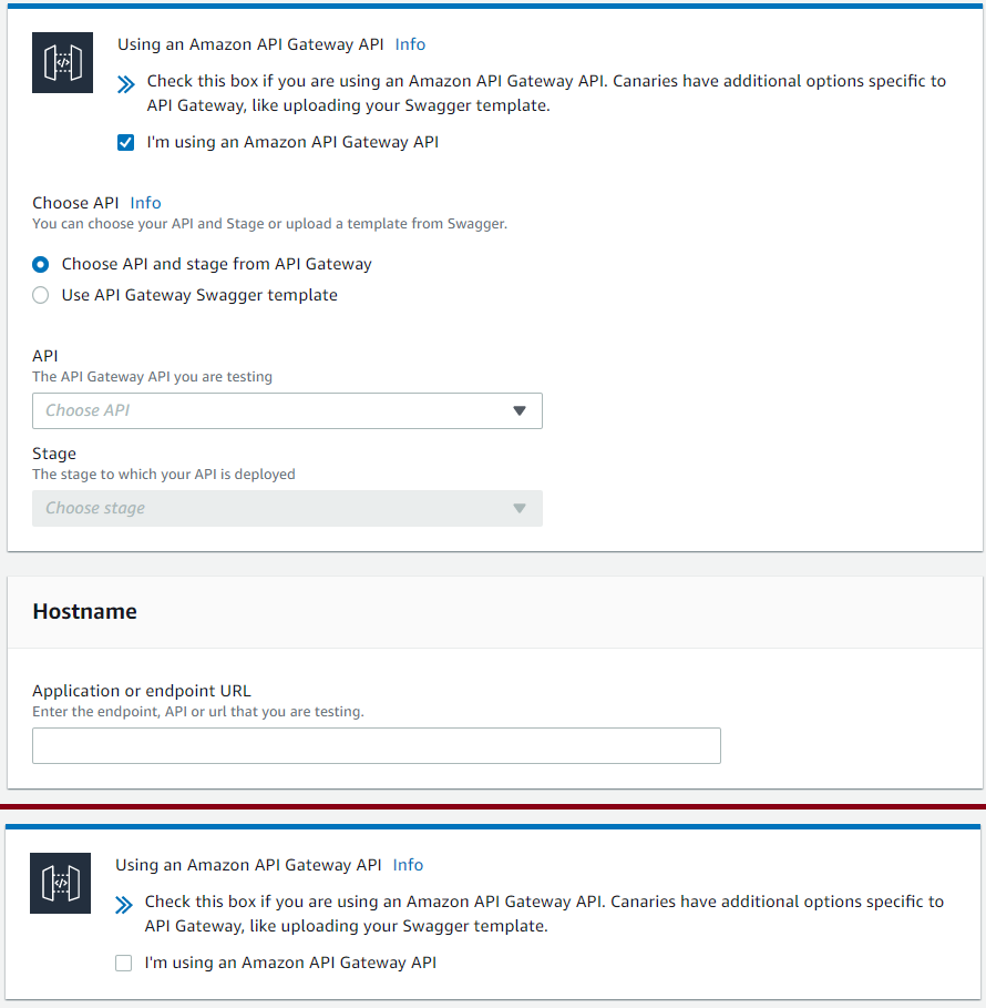
Link your Canary to an AWS API Gateway
Next, AWS gives the option to load data directly from API Gateway. If you select the checkbox, the page expands, allowing you to choose your API Gateway, stage, and Hostname. Options are loaded from what is deployed in the same AWS environment. Developers are not required to select an AWS API Gateway and can still test other endpoints with the Canaries; the information is simply loaded manually.
Setup your HTTP request
Next, add an HTTP request to your canary. If you have loaded from AWS API Gateway, a dropdown list is provided with resources attached to the endpoint. Choose the resource, method, and add any query strings or headers. If there is any authorization for your endpoint, it should be added here.
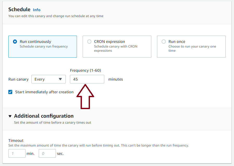
Schedule your Canary
After the HTTP setup is complete, choose the schedule for the AWS Canary. It determines how often the Canary function will hit your endpoint. You can choose between running periodically indefinitely, using a custom CRON expression, or just running the canary once. When selecting this, remember that this is adding traffic to your endpoint. This could incur costs depending on your setup.
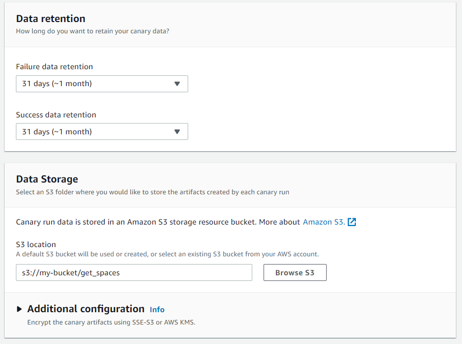
Configure log retention in AWS S3
AWS next allows developers to configure where Canary event logs are stored. They will automatically be placed into S3. From the console, developers can choose which S3 bucket should store the data and how long it should be kept. Developers can also choose to encrypt data in the S3 bucket. For exporting data to third-party tools, developers can set up a stream on the S3 bucket. This can trigger a third-party tool directly, send data via AWS Kinesis, or trigger AWS EventBridge to filter the data before sending it for analysis.
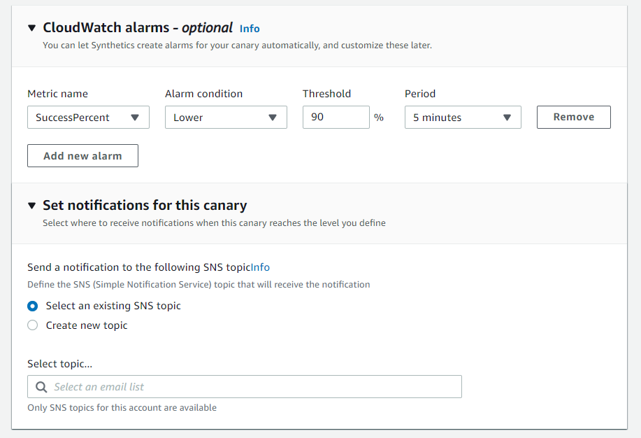
Setup an alarm
Developers can choose to set up a CloudWatch alarm on the Canary results. This is especially useful in production environments to ensure your endpoints are healthy and limit outages. The same results may also be obtained through third-party tools that enable machine learning not only to see when your endpoint has crossed a pre-set threshold but can also detect irregular or insecure events.
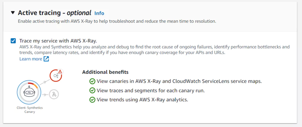
Enable AWS XRay
Developers can choose to send results of Canaries to AWS XRay. To send this data, check the box in the last section of the console screen. Enabling XRay will incur costs on your AWS account. It will also allow you another mode of observing your metrics and another path to third-party tools that can help analyze the health of your platform.
Summary
Canaries are an observability tool in AWS. Canaries give a method of analyzing API Endpoint behavior by periodically testing them and recording the results. Measured values include ensuring the endpoints are available, that returned data is expected, and that the delay in the response is within required limits.
AWS Canaries can log results to several AWS tools, including AWS Cloudwatch, AWS XRay, and AWS EventBridge. Developers can also send Canary results to third-party tools like the Coralogix platform to enable further analysis and alert DevOps teams when there are problems.
One of the benefits of deploying software on the cloud is allocating a variable amount of resources to your platform as needed. To do this, your platform must be built in a scalable way. The platform must be able to detect when more resources are required and assign them. One method of doing this is the Elastic Load Balancer provided by AWS.
Elastic load balancing will distribute traffic in your platform to multiple, healthy targets. It can automatically scale according to changes in your traffic. To ensure scaling has appropriate settings and is being delivered cost-effectively, developers need to track metrics associated with the load balancers.
Available Elastic Load Balancers
AWS elastic load balancers work with several AWS services. AWS EC2, ECS, Global Accelerator, and Route 53 can all benefit from using elastic load balancers to route traffic. Monitoring can be provided by AWS CloudWatch or third-party analytics services such as Coralogix’s log analytics platform. Each load balancer available is used to route data at a different level of the Open Systems Interconnection (OSI) model. Where the routing needs to occur strongly determines which elastic load balancer is best-suited for your system.
Application Load Balancers
Application load balancers, route events at the application layer, the seventh and highest layer of the OSI model. The load balancer component becomes the only point of contact for clients so it can appropriately route traffic. Routing can occur across multiple targets and multiple availability zones. The listener checks for requests sent to the load balancer, and routes traffic to a target group based on user-defined rules. Each rule includes a priority, action, and one or more conditions. Target groups route requests to one or more targets. Targets can include computing tasks like EC2 instances or Fargate Tasks deployed using ECS.
Developers can configure checks for target health. If this is in place, the load balancer will only be able to send requests to healthy targets, further stabilizing your system when a sufficient number of registered targets are provided.
Classic Load Balancers
Classic load balancers distribute traffic for only EC2 instances working on the transport and application OSI layers. The load balancer component is the only point of contact for clients, just as it is in application load balancers. EC2 instances can be added and removed as needed without disrupting request flows. The listener checks for requests sent to the load balancer and sends them to registered instances using a user-configured protocol and port values.
Classic load balancers can also be configured to detect unhealthy EC2 instances. They can route traffic only to healthy instances, stabilizing your platform.
Network Load Balancers
Network load balancers route events at the transport layer, the fourth layer of the OSI model. It has a very high capacity to scale requests and allows millions of requests per second. The load balancer component receives connection requests and selects targets from the user-defined ruleset. It then will open connections to selected targets on the port specified. Network load balancers handle TCP and UDP traffic using flow hash algorithms to determine individual connections.
The load balancers may be enabled to work within a certain availability zone where targets can only be registered in the same zone as the load balancer. Load balancers may also be registered as cross-zone where traffic can be sent to targets in any enabled availability zone. Using the cross-zone feature adds more redundancy and fault tolerance to your system. If targets in a single zone are not healthy, traffic is automatically directed to a different, healthy zone. Health checks should be configured to monitor and ensure requests are sent to only healthy targets.
Gateway Load Balancers
Gateway load balancers, route events at the network layer, the third layer of the OSI model. These load balancers are used to deploy, manage and scale virtual services like deep packet inspection systems and firewalls. They can distribute traffic while scaling virtual appliances with load demands.
Gateway load balancers must send traffic across VPC boundaries.They use specific endpoints set up only for gateway load balancer to accomplish this securely. These endpoints are VPC endpoints that provide a private connection between the virtual appliances in the provider VPC and the application servers in the consumer VPCs. AWS provides a list of supported partners that offer security appliances, though users are free to configure using other partners.
Metrics Available
Metrics are measured on AWS every 60 seconds when requests flow through the load balancer. No metrics will be seen if the load balancer is not receiving traffic. CloudWatch intercepts and logs the metrics. You can create manual alarms in AWS or send the data to third-party services like Coralogix, where machine learning algorithms can provide insights into the health of your endpoints.
Metrics are provided for different components of the elastic load balancers. The load balancer, target, and authorization components have their own metrics. This list is not exhaustive but contains some of the metrics considered especially useful in observing the health of your load balancer network.
Load Balancer Metrics
These metrics are all for statistics originating from the load balancers directly and do not include responses generated from targets which are provided separately.
Statistical Metrics
Load balancer metrics show how the load balancer endpoint component is functioning.
ActiveConnectionCount: The number of active TCP connections at any given time. These include connections between the client and load balancer as well as between load balancer and target. This metric should be watched to make sure your load balancer is scaling to meet your needs at any given time.
ConsumedLCUs: The number of load balancer capacity units used at any given time. This determines the cost of the load balancer and should be watched closely to track associated costs.
ProcessedBytes: The number of bytes the load balancer has processed over a period of time. This includes traffic over both IPv4 and IPv6 and includes traffic between the load balancer and clients, identity providers, and AWS Lambda functions.
HTTP Metrics
AWS provides several HTTP-specific metrics for each load balancer. Developers configure rules that determine how the load balancer will respond to incoming actions. Some of these rules will generate unique metrics so teams can count the number of events that trigger each rule type. The numbered HTTP metrics are also available from targets.
HTTP_Fixed_Response_Count: Fixed response actions return custom HTTP response codes and can include a message optionally. This metric is the number of successful fixed-response actions over a given period of time.
HTTP_Redirect_Count: Redirect actions will redirect client requests from the input URL to another. These can be temporary or permanent, depending on the setup. This metric is the number of successful redirect actions over a period of time.
HTTP_Redirect_Url_Limit_Exceeded_Count: The redirect response location is returned in the response’s header data and has a maximum size of 8K Bytes. This error metric will log the number of redirect events that failed because the URL exceeded this size limit.
HTTPCode_ELB_3XX_Count: The number of redirect codes originating from the load balancer.
HTTPCode_ELB_4XX_Count: The number of 4xx HTTP errors originating from the load balancer. These are malformed or incomplete requests that the load balancer could not forward to the target.
HTTPCode_ELB_5XX_Count: The number of 5xx HTTP errors originating from the load balancer. Internal errors in the load balancer cause these. Metrics are also available for some specific 5XX errors (500, 502, 503, and 504).
Error Metrics
ClientTLSNegotiationErrorCount: The number of connection requests initiated by the client did not connect to the load balancer due to a TLS protocol error. Issues like an invalid server certificate could cause this.
DesyncMitigationMode_NonCompliant_Request_Count: The number of requests that fail to comply with HTTP protocols
Target Metrics
Target metrics are logged for each target sent traffic from the load balancer. Targets provide all the listed HTTP code metrics provided for load balancers and those listed below.
HealthHostCount: The number of healthy targets linked to a load balancer.
RequestCountPerTarget: The average number of requests sent to a specific target in a target group. This metric applies to any target type connected to the load balancer except AWS Lambda.
TargetResponseTime: The number of seconds between when the request leaves the load balancer to when the target receives the request.
Authorization Metrics
Authorization metrics are essential for detecting potential attacks on your system. Many error metrics especially can show that nefarious calls are made against your endpoints. These metrics are critical to observe and set alarms when using Elastic load balancers.
Statistical Metrics
Some Authorization metrics are used to track the usage of the elastic load balancer. These include the following metrics
ELBAuthLatency: The time taken to query the identity provider for user information and the ID token. This latency will either be the time to return the token when successful or the time to fail.
ELBAuthRefreshTokenStatus: The number of times a refresh token is successfully used to provide a new ID token.
Error Metrics
There are three error metrics associated with authorization on elastic load balancers. Exact errors can be read in AWS Cloudwatch logs in the error_reason parameter.
ELBAuthError: This metric is used for errors such as malformed authentication actions when a connection cannot be established with the identity provider, or another internal authentication error occurred.
ELBAuthFailure: Authentication failures occur when identity provider access is denied to the user, or an authorization code is used multiple times.
ELBAuthUserClaimsSizeExceeded: This metric shows how many times the identity provider returned user claims larger than 11K Bytes. Most browsers limit cookie sizes to 4K Bytes. When a cookie is more significant than 4K, AWS ELB logs will use separate shards to handle the size. Anything up to 11K is allowed, but larger cannot be handled and will throw a 500 error.
Summary
AWS elastic load balancers scale traffic from endpoints into your platform. It allows companies to truly scale their backend and ensure the needs of their customers are always met by providing the resources needed to support those customers are available. Elastic load balancers are available for scaling at different levels of the OSI networking model.
Developers can use all or some of the available metrics to analyze the traffic flowing through and the health of their elastic load balancer setup and its targets. Separate metrics are available for the load balancer, its targets, and authorization setup. Metrics can be manually checked using AWS CloudWatch. They can also be sent to external analytics tools to alert development teams when there may be problems with the system.
Coralogix is excited to announce the launch of our Stateful Streaming Data Platform that is now available on the Red Hat Marketplace.
Built for modern architectures and workflows, the Coralogix platform produces real-time insights and trend analysis for logs, metrics, and security with no reliance on storage or indexing. Making it a perfect match for the Red Hat Marketplace.
Built-in collaboration with Red Hat and IBM, the Red Hat Marketplace delivers a hybrid multi-cloud trifecta for organizations moving into the next era of computing: a robust ecosystem of partners, an industry-leading Kubernetes container platform, and award-winning commercial support—all on a highly scalable backend powered by IBM. A private, personalized marketplace is also available through Red Hat Marketplace Select, enabling clients to provide their teams with easier access to curated software their organizations have pre-approved.
After announcing the release of Coralogix’s OpenShift operator last year the move to partnering with the Red Hat Marketplace was a giant win for Coralogix’s customers looking for an open marketplace to buy the platform.
In order to compete in the modern software market, change is our most important currency. As our rate of change increases, so too must the scope and sophistication of our monitoring system. By combining the declarative flexibility of OpenShift with the powerful analysis of Coralogix, you can create a CI/CD pipeline that enables self-healing to known and unknown issues and exposes metrics about performance. It can be extended in any direction you like, to ensure that your next deployment is a success.
“This new partnership gives us the ability to expand access to our platform for monitoring, visualizing, and alerting for more users,” said Ariel Assaraf, Chief Executive Officer at Coralogix. “Our goal is to give full observability in real-time without the typical restrictions around cost and coverage.”
With Coralogix’s OpenShift operator, customers are able to use the Kubernetes collection agents to Red Hat’s OpenShift Operator model. This is designed to make it easier to deploy and manage data from customers’ OpenShift Kubernetes clusters, allowing Coralogix to be a native part of the OpenShift platform.
“We believe Red Hat Marketplace is an essential destination to unlock the value of cloud investments,” said Lars Herrmann, Vice President, Partner Ecosystems, Product and Technologies, Red Hat. “With the marketplace, we are making it as fast and easy as possible for companies to implement the tools and technologies that can help them succeed in this hybrid multi-cloud world. We’ve simplified the steps to find and purchase tools like Coralogix that are tested, certified, and supported on Red Hat OpenShift, and we’ve removed operational barriers to deploying and managing these technologies on Kubernetes-native infrastructure.” Coralogix provides a full trial product experience via the Redhat marketplace page.
For the seasoned user, PromQL confers the ability to analyze metrics and achieve high levels of observability. Unfortunately, PromQL has a reputation among novices for being a tough nut to crack.
Fear not! This PromQL tutorial will show you five paths to Prometheus godhood. Using these tricks will allow you to use Prometheus with the throttle wide open.
Aggregation
Aggregation is a great way to construct powerful PromQL queries. If you’re familiar with SQL, you’ll remember that GROUP BY allows you to group results by a field (e.g country or city) and apply an aggregate function, such as AVG() or COUNT(), to values of another field.
Aggregation in PromQL is a similar concept. Metric results are aggregated over a metric label and processed by an aggregation operator like sum().
Aggregation Operators
PromQL has twelve built in aggregation operators that allow you to perform statistics and data manipulation.
Group
What if you want to aggregate by a label just to get values for that label? Prometheus 2.0 introduced the group() operator for exactly this purpose. Using it makes queries easier to interpret and means you don’t need to use bodges.
Count those metrics
PromQL has two operators for counting up elements in a time series. Count() simply gives the total number of elements. Count_values() gives the number of elements within a time series that have a specified value. For example, we could count the number of binaries running each build version with the query:
count_values("version", build_version)
Sum() does what it says. It takes the elements of a time series and simply adds them all together. For example if we wanted to know the total http requests across all our applications we can use:
sum(http_requests_total)
Stats
PromQL has 8 operators that pack a punch when it comes to stats.
Avg() computes the arithmetic mean of values in a time series.
Min() and max() calculate the minimum and maximum values of a time series. If you want to know the k highest or lowest values of a time series, PromQL provides topk() and bottomk(). For example if we wanted the 5 largest HTTP requests counts across all instances we could write:
topk(5, http_requests_total)
Quantile() calculates an arbitrary upper or lower portion of a time series. It uses the idea that a dataset can be split into ‘quantiles’ such as quartiles or percentiles. For example, quantile(0.25, s) computes the upper quartile of the time series s.
Two powerful operators are stddev(), which computes the standard deviation of a time series and stdvar, which computes its variance. These operators come in handy when you’ve got application metrics that fluctuate, such as traffic or disk usage.
By and Without
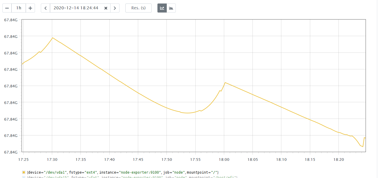
The by and without clauses enable you to choose which dimensions (metric labels) to aggregate along. by tells the query to include labels: the query sum by(instance)(node_filesystem_size_bytes) returns the total node_filesystem_size_bytes for each instance.
In contrast, withouttells the query which labels not to include in the aggregation. The query sum without(job) (node_filesystem_size_bytes) returns the total node_filesystem_size_bytes for all labels except job.
Joining Metrics
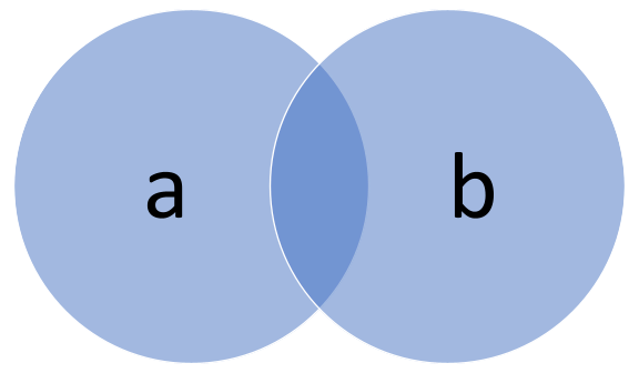
SQL fans will be familiar with joining tables to increase the breadth and power of queries. Likewise, PromQL lets you join metrics. As a case in point, the multiplication operator can be applied element-wise to two instance vectors to produce a third vector.
Let’s look at this query which joins instance vectors a and b.
a * b
This makes a resultant vector with elements a1b1, a2b2… anbn . It’s important to realise that if a contains more elements than b or vice versa, the unmatched elements won’t be factored into the resultant vector.
This is similar to how an SQL inner join works; the resulting vector only contains values in both a and b.
Joining Metrics on Labels
We can change the way vectors a and b are matched using labels. For instance, the querya * on (foo, bar) group_left(baz) b matches vectors a and b on metric labels foo and bar. (group_left(baz) means the result contains baz, a label belonging to b.
Conversely you can use ignoring to specify which label you don’t want to join on. For example the query a * ignoring (baz) group_left(baz) bjoins a and b on every label except baz. Let’s assume a contains labels foo and bar and b contains foo, bar and baz. The query will join a to b on foo and bar and therefore be equivalent to the first query.
Later, we’ll see how joining can be used in Kubernetes.
Labels: Killing Two Birds with One Metric
Metric labels allow you to do more with less. They enable you to glean more system insights with fewer metrics.
Scenario: Using Metric Labels to Count Errors
Let’s say you want to track how many exceptions are thrown in your application. There’s a noob way to solve this and a Prometheus god way.
The Noob Solution
One solution is to create a counter metric for each given area of code. Each exception thrown would increment the metric by one.
This is all well and good, but how do we deal with one of our devs adding a new piece of code? In this solution we’d have to add a corresponding exception-tracking metric. Imagine that barrel-loads of code monkeys keep adding code. And more code. And more code.
Our endpoint is going to pick up metric names like a ship picks up barnacles. To retrieve the total exception count from this patchwork quilt of code areas, we’ll need to write complicated PromQL queries to stitch the metrics together.
The God Solution
There’s another way. Track the total exception count with a single application-wide metric and add metric labels to represent new areas of code. To illustrate, if the exception counter was called “application_error_count” and it covered code area “x”, we can tack on a corresponding metric label.
application_error_count{area="x"}
As you can see, the label is in braces. If we wanted to extend application_error_count’s domain to code area “y”, we can use the following syntax.
application_error_count{area="x|y"}
This implementation allows us to bolt on as much code as we like without changing the PromQL query we use to get total exception count. All we need to do is add area labels.
If we do want the exception count for individual code areas, we can always slice application_error_count with an aggregate query such as:
count by(application_error_count)(area)
Using metric labels allows us to write flexible and scalable PromQL queries with a manageable number of metrics.
Manipulating Labels
PromQL’s two label manipulation commands are label_join and label_replace.label_join allows you to take values from separate labels and group them into one new label. The best way to understand this concept is with an example.
In this query, the values of three labels, src1, src2 and src3 are grouped into label foo. Foo now contains the respective values of src1, src2 and src3 which are a, b, and c.
label_replacerenames a given label. Let’s examine the query
This query replaces the label “service” with the label “foo”. Now foo adopts service’s value and becomes a stand in for it. One use of label_replace is writing cool queries for Kubernetes.
Creating Alerts with predict_linear
Introduced in 2015, predict_linear is PromQL’s metric forecasting tool. This function takes two arguments. The first is a gauge metric you want to predict. You need to provide this as a range vector. The second is the length of time you want to look ahead in seconds.
predict_linear takes the metric at hand and uses linear regression to extrapolate forward to its likely value in the future. As an example, let’s use PromLens to run the query:
It shows a graph which shows the predicted value an hour from the current time.
Alerts and predict_linear
The main use of predict_linear is in creating alerts. Let’s imagine you want to know when you run out of disk space. One way to do this would be an alert which fires as soon as a given disk usage threshold is crossed. For example, you might get alerted as soon as the disk is 80% full.
Unfortunately, threshold alerts can’t cope with extremes of memory usage growth. If disk usage grows slowly, it makes for noisy alerts. An alert telling you to urgently act on a disk that’s 80% full is a nuisance if disk space will only run out in a month’s time.
If, on the other hand, disk usage fluctuates rapidly, the same alert might be a woefully inadequate warning. The fundamental problem is that threshold-based alerting knows only the system’s history, not its future.
In contrast, an alert based on predict_linear can tell you exactly how long you’ve got before disk space runs out. Plus, it’ll even handle left curves such as sharp spikes in disk usage.
Scenario: predict_linear in action
This wouldn’t be a good PromQL tutorial without a working example, so let’s see how to implement an alert which gives you 4 hours notice when your disk is about to fill up. You can begin creating the alert using the following code in a file “node.rules”.
This is a PromQL expression using predict_linear. node_filesystem_free is a gauge metric measuring the amount of memory unused by your application. The expression is performing linear regression over the last hour of filesystem history and predicting the probable free space. If this is less than zero the alert is triggered.
The line after this is a failsafe, telling the system to test predict_linear twice over a 5 minute interval in case a spike or race condition gives a false positive.
Using PromQL’s predict_linear function leads to smarter, less noisy alerts that don’t give false alarms and do give you plenty of time to act.
Putting it All Together: Monitoring CPU Usage in Kubernetes
To finish off this PromQL tutorial, let’s see how PromQL can be used to create graphs of CPU-utilisation in a Kubernetes application.
In Kubernetes, applications are packaged into containers and containers live on pods. Pods specify how many resources a container can use. If a container uses more resources than its pod has, it ‘spills over’ into a second pod.
This means that a candidate PromQL query needs the ability to sum over multiple pods to get the total resources for a given container. Our query should come out with something like the following.
Container
CPU utilisation per second
redash-redis
0.5
redash-server-gunicorn
0.1
Aggregating by Pod Name
We can start by creating a metric of CPU usage for the whole system, called container_cpu_usage_seconds_total. To get the CPU utilisation per second for a specific namespace within the system we use the following query which uses PromQL’s rate function:
This is where aggregation comes in. We can wrap the above query in a sum query that aggregates over the pod name.
sum by(pod_name)( rate(container_cpu_usage_seconds_total{namespace= “redash”[5m]))
So far, our query is summing the CPU usage rate for each pod by name.
Retrieving Pod Labels
For the next step, we need to get the pod labels, “pod” and “label_app”. We can do this with the query:
group(kube_pod_labels{label_app=~”redash-*”}) by (label_app, pod)
By itself, kube_pod_labels returns all existing labels. The code between the braces is a filter acting on label_app for values beginning with “redash-”.
We don’t, however, want all the labels, just label_app and pod. Luckily, we can exploit the fact that pod labels have a value of 1. This allows us to use group() to aggregate along the two pod labels that we want. All the others are dropped from the results.
Joining Things Up
So far, we’ve got two aggregation queries. Query 1 uses sum() to get CPU usage for each pod. Query 2 filters for the label names label_app and pod. In order to get our final graph, we have to join them up. To do that we’re going to use two tricks, label_replace() and metric joining.
The reason we need label replace is that at the moment query 1 and query 2 don’t have any labels in common. We’ll rectify this by replacing pod_name with pod in query 1. This will allow us to join both queries on the label “pod”. We’ll then use the multiplication operator to join the two queries into a single vector.
We’ll pass this vector into sum() aggregating along label app. Here’s the final query:
Hopefully this PromQL tutorial has given you a sense for what the language can do. Prometheus takes its name from a Titan in Greek mythology, who stole fire from the gods and gave it to mortal man. In the same spirit, I’ve written this tutorial to put some of the power of Prometheus in your hands.
You can put the ideas you’ve just read about into practice using the resources below, which include online code editors to play with the fire of PromQL at your own pace.
This online editor allows you to get started with PromQL without downloading Prometheus. As well as tabular and graph views, there is also an “explain” view. This gives the straight dope on what each function in your query is doing, helping you understand the language in the process.
This tutorial by Coralogix explains how to integrate your Grafana instance with Coralogix, or you can use our hosted Grafana instance that comes automatically connected to your Coralogix data.
This tutorial will demonstrate how to integrate your Prometheus instance with Coralogix, to take full advantage of both a powerful open source solution and one of the most cutting edge SaaS products on the market.
Metricbeat, an Elastic Beat based on the libbeat framework from Elastic, is a lightweight shipper that you can install on your servers to periodically collect metrics from the operating system and from services running on the server. Everything from CPU to memory, Redis to NGINX, etc… Metricbeat takes the metrics and statistics that it collects and ships them to the output that you specify, such as Elasticsearch or Logstash.
In this post, we will cover some of the main use cases Metricbeat supports and we will examine various Metricbeat configuration use cases.
Metricbeat Installation
Metricbeat installation instructions can be found on the Elastic website.
Metricbeat Configuration
To configure Metricbeat, edit the configuration file. The default configuration file is called metricbeat.yml. The location of the file varies by platform. For rpm and deb, you’ll find the configuration file at this location /etc/metricbeat. There’s also a full example configuration file at /etc/metricbeat/metricbeat.reference.yml that shows all non-deprecated options.
The Metricbeat configuration file uses YAML for its syntax as it’s easier to read and write than other common data formats like XML or JSON. The syntax includes dictionaries, an unordered collection of name/value pairs, and also supports lists, numbers, strings, and many other data types.
All members of the same list or dictionary must have the same indentation level. Lists and dictionaries can also be represented in abbreviated form, which is somewhat similar to JSON using {} for dictionaries and [] for lists. For more info on the config file format.
The Modules configuration section can help with the collection of metrics from various systems.
The Processors section is used to configure processing across data exported by Metricbeat (optional). You can define a processor globally at the top-level in the configuration or under a specific module so the processor is applied to the data collected for that module.
The Output section determines the output destination of the processed data.
There are other sections you may include in your YAML such as a Kibana endpoint, internal queue, etc. You may view them and their different options at the configuring Metricbeat link. Each of the sections has different options and there are numerous module types, processors, different outputs to use, etc…
In this post, I will go over the main sections you may use and focus on giving examples that worked for us here at Coralogix.
Modules
The Modules section defines the Metricbeat input, the metrics that will be collected by Metricbeat, each module contains one or multiple metric sets. There are various module types you may use with Metricbeat, you can configure modules in the modules.d directory (recommended), or in the Metricbeat configuration file. In my examples, I’ll configure the module in the Metricbeat configuration file. Here is an example of the System module. For more info on configuring modules and module types.
#============================= Metricbeat Modules =============================
metricbeat.modules:
- module: system
  metricsets:
    - cpu # CPU usage
    - load # CPU load averages
    - memory # Memory usage
    - network # Network IO
    #- core # Per CPU core usage
    #- diskio # Disk IO
    #- filesystem # File system usage for each mountpoint
    #- fsstat # File system summary metrics
    #- raid # Raid
    #- socket # Sockets and connection info (linux only)
    #- service # systemd service information
  enabled: true
  period: 10s
There are some more options to this module type as you can observe in the full example config file. These are all the available metric sets with the system module type, the enable parameter is optional, by default if not specified it is set to true and the period parameter is setting how often the metric sets are executed. This setting is required for all module types. You may include multiple module types, all in the same YAML configuration. If you are working with Coralogix and wish to send your metrics to your Coralogix account you will have to include the fields parameter with our required fields, this is beside the fact you need to choose our Logstash endpoint in your config output, we will see a similar example later.
Processors
You can use Processors in order to process events before they are sent to the configured output. The libbeat library provides processors for reducing the number of exported fields, performing additional processing and decoding, etc… Each processor receives an event, applies a defined action to the event, and returns the event. If you define a list of processors, they are executed in the order they are defined in the configuration file. This is an example of several processors configured. For more information on filtering and enhancing your data.
# ================================= Processors =================================
# Processors are used to reduce the number of fields in the exported event or to
# enhance the event with external metadata. This section defines a list of
# processors that are applied one by one and the first one receives the initial
# event:
#
# event -> filter1 -> event1 -> filter2 ->event2 ...
#
# The supported processors are drop_fields, drop_event, include_fields,
# decode_json_fields, and add_cloud_metadata.
#
# For example, you can use the following processors to keep the fields that
# contain CPU load percentages, but remove the fields that contain CPU ticks
# values:
#
processors:
- include_fields:
fields: ["cpu"]
- drop_fields:
fields: ["cpu.user", "cpu.system"]
#
# The following example drops the events that have the HTTP response code 200:
#
processors:
- drop_event:
when:
equals:
http.code: 200
#
# The following example renames the field a to b:
#
processors:
- rename:
fields:
- from: "a"
to: "b"
#
# The following example enriches each event with the machine's local time zone
# offset from UTC.
#
processors:
- add_locale:
format: offset
#
# The following example enriches each event with host metadata.
#
processors:
- add_host_metadata: ~
#
# The following example decodes fields containing JSON strings
# and replaces the strings with valid JSON objects.
#
processors:
- decode_json_fields:
fields: ["field1", "field2", ...]
process_array: false
max_depth: 1
target: ""
overwrite_keys: false
#
# The following example copies the value of message to message_copied
#
processors:
- copy_fields:
fields:
- from: message
to: message_copied
fail_on_error: true
ignore_missing: false
#
# The following example preserves the raw message under event_original, which then cut at 1024 bytes
#
processors:
- copy_fields:
fields:
- from: message
to: event_original
fail_on_error: false
ignore_missing: true
- truncate_fields:
fields:
- event_original
max_bytes: 1024
fail_on_error: false
ignore_missing: true
#
# The following example URL-decodes the value of field1 to field2
#
processors:
- urldecode:
fields:
- from: "field1"
to: "field2"
ignore_missing: false
fail_on_error: true
#
# The following example is a great method to enable sampling in Metricbeat, using Script processor#
processors:- script:
lang: javascript
id: my_filter
source:>function process(event){if(Math.floor(Math.random()*100)<50){event.Cancel();}}
Metricbeat offers more types of processors as you can see here and you may also include conditions in your processor definition. If you use Coralogix, you have an alternative to Metricbeat Processors, to some extent, as you can set different kinds of parsing rules through the Coralogix UI instead. If you are maintaining your own ELK stack or other 3rd party logging tool you should check for processors when you have any need for parsing.
Output
You configure Metricbeat to write to a specific output by setting options in the Outputs section of the metricbeat.yml config file. Only a single output may be defined. In this example, I am using the Logstash output. This is the required option if you wish to send your logs to your Coralogix account, using Metricbeat. For more output options.
# ================================= Logstash Output =================================
output.logstash:
  # Boolean flag to enable or disable the output module.
  enabled: true

  # The Logstash hosts
  hosts: ["localhost:5044"]

  # Configure escaping HTML symbols in strings.
  escape_html: true

  # Number of workers per Logstash host.
  worker: 1

  # Optionally load-balance events between Logstash hosts. Default is false.
  loadbalance: false

  # The maximum number of seconds to wait before attempting to connect to
  # Logstash after a network error. The default is 60s.
  backoff.max: 60s

  # Optional index name. The default index name is set to filebeat
  # in all lowercase.
  index: 'filebeat'

  # The number of times to retry publishing an event after a publishing failure.
  # After the specified number of retries, the events are typically dropped.
  # Some Beats, such as Filebeat and Winlogbeat, ignore the max_retries setting
  # and retry until all events are published.  Set max_retries to a value less
  # than 0 to retry until all events are published. The default is 3.
  max_retries: 3

  # The maximum number of events to bulk in a single Logstash request. The
  # default is 2048.
  bulk_max_size: 2048

  # The number of seconds to wait for responses from the Logstash server before
  # timing out. The default is 30s.
  timeout: 30s
This example only shows some of the configuration options for the Logstash output, there are more. It’s important to note that when using Coralogix, you specify the following Logstash host: logstashserver.coralogixstg.wpengine.com:5044 under hosts and that some other options are redundant, such as index name, as it is defined by us.
At this point, we have enough Metricbeat knowledge to start exploring some actual configuration files. They are commented and you can use them as references to get additional information about different plugins and parameters or to learn more about Metricbeat.
Metricbeat Configuration Examples
Example 1
This example uses the system module to monitor your local server and send different metric sets. The Processors section includes a processor to drop unneeded beat metadata. The chosen output for this example is stdout.
This example uses the system module to monitor your local server and send different metric sets, forwarding the events to Coralogix’s Logstash server (output) with the secured connection option. The Processors section includes a processor to sample the events to send 50% of the data.
#============================= Metricbeat Modules =============================
metricbeat.modules:
- module: system
  metricsets:
    - cpu             # CPU usage
    - load            # CPU load averages
    - memory          # Memory usage
    - network         # Network IO
  enabled: true
  period: 10s
#============================= General =============================
fields_under_root: true
fields:
  PRIVATE_KEY: "XXXXXXXX-XXXX-XXXX-XXXX-XXXXXXXXXXXX"
  COMPANY_ID: XXXXX
  APP_NAME: "metricbeat"
  SUB_SYSTEM: "system"
#================================= Processors =================================
processors:
# The following example is a great method to enable sampling in Filebeat, using Script processor. This script processor drops 50% of the incoming events
  - script:
      lang: javascript
      id: my_filter
      source: >
        function process(event) {
            if (Math.floor(Math.random() * 100) < 50) {
              event.Cancel();
            }
        }
#================================= Logstash output =================================
output.logstash:
  enabled: true
  hosts: ["logstashserver.coralogixstg.wpengine.com:5015"]
  ssl.certificate_authorities: ["/var/log/metricbeat/ca.crt"]
Be Our Partner
Complete this form to speak with one of our partner managers.
Thank You
Someone from our team will reach out shortly. Talk to you soon!
 The new standard of observability is here. Discover Olly, the industry’s first