
Ship OpenTelemetry Data to Coralogix via Reverse Proxy (Caddy 2)
It is commonplace for organizations to restrict their IT systems from having direct or unsolicited access to external networks or the Internet, with network proxies serving…

Out of the four basic computing resources (storage, memory, compute, network), storage tends to be positioned as the foremost one to focus on for any architect optimizing an Elasticsearch cluster. Let’s take a closer look at a couple of interesting aspects in relation to the Elasticsearch storage optimization and let’s do some hands-on tests along the way to get actionable insights.
The storage topic consists of two general perspectives:
| OPTIMIZATION | PROS | CONS | BEST FOR |
| Defaults everything on default | — | The indexed size of data expands by ~20% (compared to 100MB of raw JSON data) | Initial setup or unknown specific patterns |
| Mapping Based Disable storing of normalization factors and positions in string fields | Reduction in size compared to defaults by ~11% | We lose the ability to score on phrase queries and score on a specific field | Non-Fulltext setups |
| Mapping Based Store all string fields only as keywords | Reduction in size by ~30% (to defaults) and ~20% (compared to raw data) | We lose the option to run full-text queries ie left with exact matching | Non-Fulltext setups with fully structured data where querying involves only filtering, aggregations and term-level matching. |
| Settings Based Keywords-only mapping, more efficient compression scheme (DEFLATE as opposed to the default of LZ4) | Further reduction in size by ~14% (~44% compared to defaults and ~32% compared to raw) | Minor speed loss (higher CPU load) | Same as above with even more focus on stored data density |
| Mapping Based Disable storing _source field, after forcemerge | Reduction in size by ~50% compared to raw data | We lose the ability to use update, update_by_query and especially reindex APIs | Just experimental setups (not recommended) |
| Shards Based Forcemerge all our previous indices | Reduction in size compared to raw baseline by another ~1-15% (this can vary a lot) | We lose the option to continue to write in the indices efficiently | Setups with automatically rolled indices (where read-only ones can be forcemerged to be more space-efficient) |
Depending on your deployment model you’ll be (to some extent) likely to confront decisions around the physical characteristics of your storage layer so let’s start here. Obviously, when you are spinning up a fully managed service instance you won’t have to worry about what specific drives are under the hood (like you would in your data center or some IaaS platform) but at least at the conceptual level, you will likely be facing the decision to pick SSDs or HDDs for your nodes. The recipe that is usually suggested is quite simple: choose SSDs for ingesting and querying the freshest, most accessed data where the mixed read/write flows and their latency is the primary factor or if you have no deeper knowledge about the overall requirements, i.e. the “default” option. For logs and time-series data, this storage will likely be the first week or two of the lifecycle of your data. Then, at a later phase where (milli)seconds of a search latency is not a major concern, but rather to keep a longer history of your indexed data efficiently, you can choose server-class HDDs as the price:space ratio is still slightly better. The usual resource-requirement patterns in these setups are the following:
| Side note: remember that the success of any resource-related decision in the ES world relies heavily on good knowledge of your use-case (and related access patterns and data flows) and can be highly improved by “real-life” data from benchmarking and simulations. Elastic offers a special tool for this called Rally, and published 7 tips for better benchmarks (to ensure validity, consistency, and reproducibility of the results) and runs a couple of regular benchmarks on its own (as well as some published by others). |
RAID is another topic frequently discussed on Elastic discussion forums as it is usually required in enterprise datacenters. Generally, RAID is optional given the default shards replication (if correctly set up eg. not sharing specific underlying resources) and the decision is driven by whether you want to handle this at the hardware level as well. RAID0 can improve performance but should be kept in pairs only (to keep your infra ops sane). Other RAID configurations with reasonable performance (from the Write perspective for example 1/10) are acceptable but can be costly (in terms of a redundant space used), while RAID5 (though very usual in data centers) tends to be slow(ish).
Besides RAID, you also have the option to use multiple data paths to link your data volumes (in the elasticsearch.yml path.data). This will result in the distribution of shards across the paths with one shard always in one path only (which is ensured by ES). This way you can achieve a form of data striping across your drives and parallel utilization of multiple drives (when sharding is correctly set up). ES will handle the placement of replica shards on different nodes from the primary shard.
If you are dealing with a continuous flow of time series data (logs, metrics, events, IoT, telemetry, messaging, etc) you will likely be heading towards a so-called hot-warm(-cold) architecture where you gradually move and reshape your indexes, mostly based on time/size conditions, to accommodate for continuously changing needs (as previously outlined in the usual resource-requirement patterns). This can all be happening on nodes with non-uniform resource configurations (not just from the storage perspective but also the memory and CPU perspective, etc.) to achieve the best cost to performance ratio. 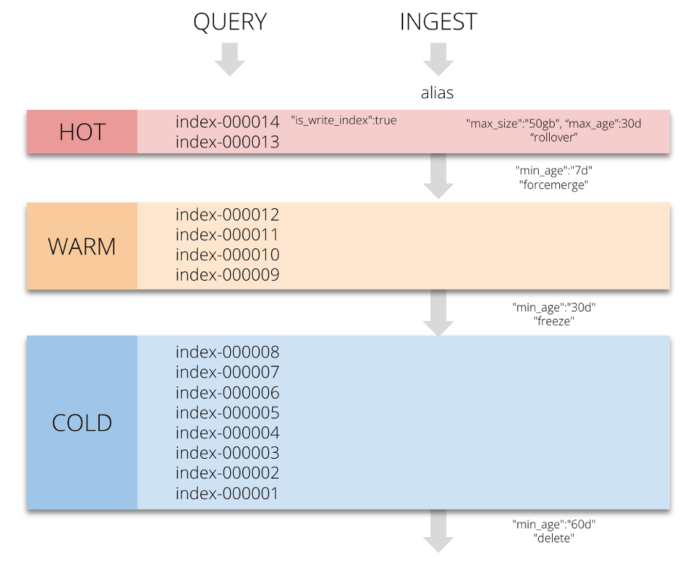 To achieve this we need to be able to automatically and continually move the shards between nodes that have different resource characteristics based on preset conditions. For example, placing shards of a newly created index on HOT nodes with SSDs and then after 14 days, moving those shards away from the HOT nodes to long term storage to make space for fresher data on the more performant hardware). There are three complementary Elasticsearch instruments that come handy for this situation:
| Side Notes: 1. you can review your existing tags using the _cat/nodeattrs API, 2. you can use the same shard allocation mechanism globally at the cluster-level to be able to define global rules for any new index that gets created. |
Sounds fun… let’s use these features! You can find all of the commands/requests and configurations in the repo below (hands-on-1-nodes-tiering dir). All commands are provided as shell script files so you can launch them one after another ./tiering/1_ilm_policy.sh ./tiering/2…
| Link to git repo: https://github.com/coralogix-resources/wikipedia_api_json_data |
As our test environment, we’ll use a local Docker with the docker-compose.yml file that will spin-up a four-node cluster running in containers on localhost (complemented with Kibana to inspect it via the UI). Take a look and clone the repo!
Important: In this article, we won’t explain Docker or a detailed cluster configuration (you can check out this article for a deep-dive) because for our context, the valid part is only the node tagging. In our case, we’ll define the specific node tags via the environment variables in the docker-compose.yml file that gets injected into the container when it started. We will use these tags to distinguish between our hypothetical hot nodes (with a stronger performance configuration, consisting of the most recent data) as well as warm nodes to ensure long term denser storage:
environment:
 - node.attr.type=warm
“Normally” you would do it in a related elasticsearch.yml file of the node.
echo "node.attr.type: hot" >> elasticsearch.yml
Now that we have our cluster running and nodes categorized (ie tagged), we’ll define a very simple index lifecycle management (ILM) policy which will move the index from one type of node (tagged with the custom “type” attribute) to another type of node after a predefined period. We’ll operate at one-minute intervals for this demo, but in real life, you would typically configure the interval in ‘days’. Here we’ll move any index managed by this policy to a ‘warm’ phase (ie running on the node with the ‘warm’ tag) after an index age of 1 minute:
#!/bin/bash
curl --location --request PUT 'http://localhost:9200/_ilm/policy/elastic_storage_policy' \
--header 'Content-Type: application/json' \
--data-raw '{
   "policy": {
       "phases": {
           "warm": {
               "min_age": "1m",
               "actions": {
                   "allocate": {
                       "require": {
                           "type": "warm"
                       }
                   }
               }
           }
       }
   }
}
Because the ILM checks for conditions that are fulfilled every 10 minutes by default, we’ll use a cluster-level setting to bring it down to 1 minute.
#!/bin/bash
curl --location --request PUT 'http://localhost:9200/_cluster/settings' \
--header 'Content-Type: application/json' \
--data-raw '{
   "transient": {
       "indices.lifecycle.poll_interval": "1m"
   }
}'
REMEMBER: If you do this on your cluster, do not forget to bring this setting back up to a reasonable value (or the default) as this operation can be costly when having lots of indices.
Now let’s create an index with 2 shards (primary and replica), which is ILM managed and that we will force onto our hot nodes via index.routing.allocation.require and the defined custom type attribute of hot.
#!/bin/bash
curl --location --request PUT 'http://localhost:9200/elastic-storage-test' \
--header 'Content-Type: application/json' \
--data-raw '{
   "settings": {
       "number_of_shards": 1,
       "number_of_replicas": 1,
       "index.lifecycle.name": "elastic_storage_policy",
       "index.routing.allocation.require.type": "hot"
   }
}'
Now watch carefully… immediately after the index creation, we can see that our two shards are actually occupying the hot nodes of esn01 and esn02. curl localhost:9200/_cat/shards/elastic-storage*?v index shard prirep state docs store ip node elastic-storage-test 0 p STARTED 0 230b 172.23.0.2 esn02 elastic-storage-test 0 r STARTED 0 230b 172.23.0.4 esn01 … but if we wait up to two minutes (imagine here two weeks :)) we can see that the shards were reallocated to warm nodes as we required in the ILM policy.
curl localhost:9200/_cat/shards/elastic-storage*?v
index                shard prirep state   docs store ip         node
elastic-storage-test 0     p      STARTED    0  230b 172.23.0.5 esn03
elastic-storage-test 0     r      STARTED    0  230b 172.23.0.3 esn04
If you want to know more, you can check the current phase and the status of a life-cycle for any index via the _ilm/explain API.
curl localhost:9200/elastic-storage-test/_ilm/explain?pretty
Optional: if you don’t want to use the ILM automation you can reallocate/reroute the shards manually (or via scripts) with the index/_settings API and the same attribute we have used when creating the index. For example:
#!/bin/bash
curl --location --request PUT 'http://localhost:9200/elastic-storage-test/_settings' \
--header 'Content-Type: application/json' \
--data-raw '{
 "index.routing.allocation.require.type": "warm"
}'
Perfect! Everything went smoothly, now let’s dig a little deeper.
Now that we went through the drives and the related setup we should take a look at the second part of the equation; the data that actually resides on our storage. You all know that ES expects indexed documents to be in JSON format, but to allow for its many searching/filtering/aggregation/clustering/etc. capabilities, this is definitely not the only data structure stored (and it doesn’t even have to be stored as you will see later).

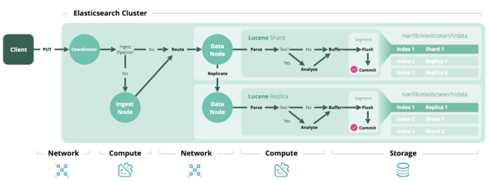
Indexing in action (image source elastic.co).
As described in the ES docs the following data gets stored on disk for the two primary roles that an individual node can have (data & master-eligible):
Data nodes maintain the following data on disk:
Master-eligible nodes maintain the following data on disk:
|
If we try to uncover what’s behind the shard data we will be entering the waters of Apache Lucene and the files it maintains for its indexes… so definitely a todo: read more about Lucene as it is totally interesting 🙂
The Lucene docs have a nice list of files it maintains for each index (with links to details):
| Name | Extension | Brief Description |
| Segments File | segments_N | Stores information about a commit point |
| Lock File | write.lock | The Write lock prevents multiple IndexWriters from writing to the same file. |
| Segment Info | .si | Stores metadata about a segment |
| Compound File | .cfs, .cfe | An optional “virtual” file consisting of all the other index files for systems that frequently run out of file handles. |
| Fields | .fnm | Stores information about the fields |
| Field Index | .fdx | Contains pointers to field data |
| Field Data | .fdt | The stored fields for documents |
| Term Dictionary | .tim | The term dictionary, stores term info |
| Term Index | .tip | The index into the Term Dictionary |
| Frequencies | .doc | Contains the list of docs which contain each term along with the frequency |
| Positions | .pos | Stores position information about where a term occurs in the index |
| Payloads | .pay | Stores additional per-position metadata information such as character offsets and user payloads |
| Norms | .nvd, .nvm | Encodes length and boost factors for docs and fields |
| Per-Document Values | .dvd, .dvm | Encodes additional scoring factors or other per-document information. |
| Term Vector Index | .tvx | Stores offset into the document data file |
| Term Vector Data | .tvd | It contains term vector data. |
| Live Documents | .liv | Info about what documents are live |
| Point values | .dii, .dim | Holds indexed points, if any |
Significant concepts for the Lucene data structures are as follows:
Significant concepts for the ES part of things are the following structures:
So these were the actual data structures and files that both of the involved software components (Elasticsearch and Lucene) are storing. Another important factor in relation to stored data structures and generally the resulting storage efficiency is the shard size. The reason is that as we have seen there are lots of overhead data structures and maintaining them can be “disk-space-costly” so a general recommendation is to use large shards and by large it means at the scale of GB – somewhere up to 50 GB. So try to aim for this sizing instead of a large number of small indexes/shards, which quite often happens when the indices are created on a daily basis. Enough talking, let’s get our hands dirty.
When we inspect the ES docs in relation to the tuning of the disk usage, we find the recommendation to start with optimizations of mappings you use, then proposing some setting-based changes and finally shard/index-level tuning. It could be quite interesting to see the actual quantifiable impacts (still only indicative though) of changing some of these variables. Sounds like a plan!
| Data sidenote: for quite a long time I’ve been looking for reasonable testing data for my own general-testing with ES that would offer a combination of short term fields, text fields, some number values etc. So far, the closest I got is with the Wikipedia REST API payloads, especially with the /page/summary (which gives you the key info for a given title) and the /page/related endpoint which gives you summaries for 20 pages related to the given page. We’ll use it in this article… one thing I want to highlight is that the wiki REST API is not meant for large data dumping (but more for app-level integrations) so use it wisely and if you need more use, try the full-blown data dump and you will have plenty of data to play with. |
For this hands-on, I wrote a Python script that:
As this is not a Python article we won’t go into much of the inner details (maybe we can do it another time). You can find everything (code, scripts, requests, etc.) in the linked repo in hands-on-2-index-definition-size-implications and code folders. The code is quite simple just to fulfill our needs (so feel free to improve it for yourself).
| Link to git repo: https://github.com/coralogix-resources/wikipedia_api_json_data |
Provided are also reference data files with downloaded content related to the “big four” tech companies “Amazon”, “Google”, “Facebook”, and “Microsoft”. We’ll use exactly this dataset in the hands-on test so this will be our BASELINE of ~100MB in raw data (specifically 104858679 bytes, with 38629 JSON docs). The wiki.data file is the raw JSON data and the series of wiki_n.bulk files are the individual chunks for the _bulk API
ls -lh data | awk '{print $5,$9}'
100M wiki.data
10M wiki_1.bulk
10M wiki_2.bulk
11M wiki_3.bulk
10M wiki_4.bulk
11M wiki_5.bulk
10M wiki_6.bulk
10M wiki_7.bulk
11M wiki_8.bulk
10M wiki_9.bulk
6.8M wiki_10.bulk
We’ll use a new single-node instance to start fresh and we’ll try the following:
Important: don’t do this on indexes that are still being written to (ie only do it on read-only indexes). Also, note that this is quite an expensive operation (so not to be done during your peak hours). Optionally you can also complement this with the _shrink API to reduce the number of shards.
Creating the index: the only thing we will configure is that we won’t use any replica shards as we are running on a single node (so it would not be allocated anyways) and we are just interested in the sizing of the primary shard.
#!/bin/bash
curl --request PUT 'http://localhost:9200/test-defaults' \
--header 'Content-Type: application/json' \
-d '{
   "settings": {
       "number_of_shards": 1,
       "number_of_replicas": 0
   }
}'
Now, let’s index our data with
./_ES_bulk_API_curl.sh ../data test-defaults
As this is the first time indexing our data, let’s also look at the indexing script which is absolutely simple.
#!/bin/bash
for i in $1/*.bulk; do curl --location --request POST "http://localhost:9200/$2/_doc/_bulk?refresh=true" --header 'Content-Type: application/x-ndjson' --data-binary "@$i"; done
Let it run for a couple of seconds.. and the results are…
curl 'localhost:9200/_cat/indices/test*?h=i,ss'
test-defaults 121.5mb
Results: Our latest data is inflated compared to the original raw data by more than 20% (i.e. 100MB of JSON data compared to 121.5MB).
Interesting!
Note: if you are not using the provided indexing script but are testing with your specific data, don’t forget to use the _refresh API to see fully up-to-date sizes/counts (as the latest stats might not be shown).
curl 'localhost:9200/test-*/_refresh' |
Now we are going to disable storing of normalization factors and positions using the norms and index_options parameters. To apply these settings on all textual fields (no matter how many there are) we’ll use dynamic_templates (this should not be mistaken with standard index templates). Dynamic templates allow you to dynamically apply mappings by automatically matching data types (in this case, strings).
#!/bin/bash
curl --request PUT 'http://localhost:9200/test-norms-freqs' \
--header 'Content-Type: application/json' \
-d '{
   "settings": {
       "number_of_shards": 1,
       "number_of_replicas": 0
   },
   "mappings": {
       "dynamic_templates": [
           {
               "strings": {
                   "match_mapping_type": "string",
                   "mapping": {
                       "type": "text",
                       "norms": false,
                       "index_options": "freqs",
                       "fields": {
                           "keyword": {
                               "type": "keyword",
                               "ignore_above": 256
                           }
                       }
                   }
               }
           }
       ]
   }
}'
and then we index…
./_ES_bulk_API_curl.sh ../data test-norms-freqs
Results: Now we are down by ~11% compared to storing the normalization factors and positions but still we’re above the size of our raw baseline.
test-norms-freqs   110mb
test-defaults    121.5mb
If you are working with mostly structured data, then you may find yourself in a position that you don’t need full-text search capabilities in your textual fields (but still want to keep the option to filter, aggregate etc.). In this situation, it’s reasonable to use just the keyword type in mapping.
#!/bin/bash
curl --request PUT 'http://localhost:9200/test-keywords' \
--header 'Content-Type: application/json' \
-d '{
   "settings": {
       "number_of_shards": 1,
       "number_of_replicas": 0
   },
   "mappings": {
       "dynamic_templates": [
           {
               "strings": {
                   "match_mapping_type": "string",
                   "mapping": {
                       "type": "keyword",
                       "ignore_above": 256
                   }
               }
           }
       ]
   }
}'
Results: (you know how to index the data by now :)) Below, we improved our baseline performance by almost 20% (and ~30% compared to the default configuration)! Especially in the logs processing area (if carefully evaluated per field) there can be lots of space-saving potential with this configuration.
test-norms-freqs   110mb
test-defaults    121.5mb
test-keywords     81.1mb
Now we are going to test a more efficient compression algorithm (DEFLATE) by setting “index.codec” to “best_compression”. Let’s keep the previous mapping to see how much further we can push it.
#!/bin/bash
curl --request PUT 'http://localhost:9200/test-compression' \
--header 'Content-Type: application/json' \
-d '{
   "settings": {
...
       "index.codec": "best_compression"
   },
...
'
Results: we got another ~14% further performance improvement compared to the baseline which is significant (ie approx. 44% down compared to defaults and 32% compared to raw)! We might experience some performance slowdowns on queries, but if we are in the race of fitting as much data as possible, then this is a killer option.
test-compression  68.2mb
test-norms-freqs   110mb
test-defaults    121.5mb
test-keywords     81.1mb
Up until this point I find the changes we have realized “reasonable” (obviously you need to evaluate your specific conditions/needs). The following optimization I would not definitely recommend in production setups (as will lose the option to use the reindex API among other things) but let’s see how much of the remaining space the removal of the _source field may save.
#!/bin/bash
curl --request PUT 'http://localhost:9200/test-source' \
--header 'Content-Type: application/json' \
-d '{
...
   "mappings": {
       "_source": {
           "enabled": false
       },
...
Results: It somehow didn’t change almost anything… weird! But let’s wait a while… maybe something will happen after the next step (forcemerge). Spoiler alert: it will.
test-compression  68.2mb
test-norms-freqs   110mb
test-defaults    121.5mb
test-keywords     81.1mb
test-source         68mb
_forcemerge allows us to merge segments in shards to reduce the number of segments and related overhead data structures. Now let’s first see how many segments one of our previous indexes had to know if merging them might help reduce the data size. For the inspection, we will use the _stats API which is super-useful for getting insights both at the indices-level as well as the cluster-level.
curl 'localhost:9200/test-defaults/_stats/segments' | jq
We can see that we have exactly 14 segments + other useful quantitative data about our index.
{
   "test-defaults": {
       "uuid": "qyCHCZayR8G_U8VnXNWSXA",
       "primaries": {
           "segments": {
               "count": 14,
               "memory_in_bytes": 360464,
               "terms_memory_in_bytes": 245105,
               "stored_fields_memory_in_bytes": 22336,
               "term_vectors_memory_in_bytes": 0,
               "norms_memory_in_bytes": 29568,
               "points_memory_in_bytes": 2487,
               "doc_values_memory_in_bytes": 60968,
               "index_writer_memory_in_bytes": 0,
               "version_map_memory_in_bytes": 0,
               "fixed_bit_set_memory_in_bytes": 0,
               "max_unsafe_auto_id_timestamp": -1,
               "file_sizes": {}
           }
       }
   }
}
So let’s try force-merging the segments on all our indices (from whatever number they currently have into one segment per shard) with this request:
curl --request POST 'http://localhost:9200/test-*/_forcemerge?max_num_segments=1'
| Note that during the execution of the force merge operation, the number of segments can actually rise before settling to the desired final value (as there are new segments that get created while reshaping the old ones). |
Results: When we check our index sizes we find that the merging helped us optimize again by reducing the storage requirements. But the extent differs… about a further ~1-15% reduction as it is very tightly coupled with specifics of the data structures that are actually stored (where some of these were removed for some of the indices in the previous steps). Also, the result is not really representative since our testing dataset is quite small, but with bigger data, you can likely expect more storage efficiency. I, therefore, consider this option to be very useful.
test-compression  66.7mb
test-norms-freqs 104.9mb
test-defaults    113.5mb
test-keywords       80mb
test-source       50.8mb
| Note: now you can see the impact of the forcemerging on the index without the _source field stored. |
As the last optimization step, we can check out the actual files in the ES container. Let’s review the disk usage in the indices dir (under /usr/share/elasticsearch) where we find each of our indexes in separate subdirectories (identified by UUID). And as you can see the numbers are aligned (+/- 1MB) with the sizes we received via API.
docker exec -it elastic /bin/bash
du -h ./data/nodes/0/indices/ --max-depth 1
105M	./data/nodes/0/indices/5hF3UTaPSl-O4jIMRgxtnQ
114M	./data/nodes/0/indices/qyCHCZayR8G_U8VnXNWSXA
67M	./data/nodes/0/indices/JQbpknJGRAqpbi7sckoVqQ
51M	./data/nodes/0/indices/u0R57ilFSeOg0r0KVoFh0Q
81M	./data/nodes/0/indices/eya3KsEeTO27HiYcrqYIFg
417M	./data/nodes/0/indices/
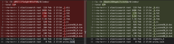
To see the data files of Lucene we have previously discussed just go further in the tree. We can, for example, compare the size of the last two indexes (with and without _source field). We can see the biggest difference is on the .fdt Lucene file (i.e. stored field data).
That’s it… what a ride!
In this article, we have reviewed two sides of Elasticsearch storage optimization. In the first part, we have discussed individual options related to the drives and data storage setups and we actually tested out how to move our index shards across different tiers of our nodes reflecting different types of drives or node performance levels. This can serve as a basis for the hot-warm-cold architectures and generally supports the efficient use of the hardware we have in place. In the second part, we took a closer look at actual data structures and files that Elasticsearch maintains and through a multistep hands-on optimization process, we reduced the size of our testing index by almost 50%.

It is commonplace for organizations to restrict their IT systems from having direct or unsolicited access to external networks or the Internet, with network proxies serving…

What is AWS Systems Manager Before we jump into this, it’s important to note that older names, and still in use in some areas of AWS,…

Infrastructure as Code is an increasingly popular DevOps paradigm. IaC has the ability to abstract away the details of server provisioning. This tutorial will look at…